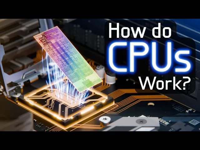
The Engineering that Runs the Digital World 🛠️⚙️💻 How do CPUs Work?

0:00 Inside every desktop computer, smartphone, gaming console, laptop,

0:05 or practically any other device you use on a daily

0:09 basis is a CPU or Central Processing Unit,

0:12 and in this video, we’re going to see how they work.

0:16 A typical processor for a powerful laptop like

0:19 this one is built from billions of nanoscopic

0:23 transistors connected together using dozens of layers of wires

0:27 and is essentially the brain of the device.

0:31 But before we explore the microprocessor and all its complexity,

0:35 let’s travel to the early days of personal computers and video game

0:40 consoles and compare the Apple 2e from 1983 to the modern-day MacBook Pro.

0:46 Inside the Apple 2e we find a chip called a 6502,

0:51 which is considered one of the great-grandparents of all modern processors.

0:56 This chip is built from 4528 transistors

1:00 and can perform around 430 thousand calculations a second.

1:06 While it could only run primitive

1:09 applications and video games with simple graphics,

1:12 this chip was the backbone of a generation of early

1:16 computers and video game consoles such as the NES,

1:19 the Commodore 64, and the Atari.

1:22 Compare that to the MacBook Pro’s M1 processor which is built

1:27 from 16 billion transistors capable of performing

1:31 around 3 trillion calculations a second,

1:35 thus enabling it to generate expansive 3D worlds with immersive graphics.

1:41 Despite these two chips being released around 45 years apart,

1:45 the underlying principles of how they work are rather similar.

1:49 In a way, you can think of these devices

1:51 as sharing a common section of technological DNA.

1:54 In fact, if we were to open up a desktop computer

1:58 and grab the CPU or the GPU inside the graphics card,

2:03 or teardown a Nintendo Switch or Smartphone

2:05 and find the system on a chip or SoC, or even if you could make your way

2:12 into an AI Data Center and grab a state-of-the-art AI chip,

2:16 you’d find that all of these processors

2:19 operate using the same underlying principles.

2:23 In other words, both the Oregon Trail of 50 years ago

2:27 and advanced AI algorithms run on processors with similar technological DNA,

2:33 but of course, one of these chips is

2:37 10 billion times more computationally powerful than the other.

2:41 So, in this video, we’re going to take apart this microprocessor and find out

2:46 exactly what the shared technological DNA is and how it enables CPUs to work.

2:52 And just to be clear,

2:54 the technological DNA is not transistors and it’s not logic gates,

3:00 but rather it’s an architectural design and basic operational principle that’s

3:07 fundamental to microprocessors and differentiates

3:10 these chips from other integrated circuits.

3:14 So, stick around, and let’s dive right in.

3:24 This video is sponsored by Brilliant.

3:27 Let’s begin with a quick 3D animated teardown of this Macbook Pro.

3:32 When we open it up, we find

3:35 a range of different components such as the touchpad,

3:38 battery cells, speakers, a cooling fan, and the motherboard in the center.

3:44 Mounted to the motherboard are the solid state drive or SSD Storage

3:49 chips where all your files are saved and a range of other chips.

3:54 Underneath the heat pipe, we find the DRAM which is the short

3:58 term working memory and central processing unit.

4:01 Let’s desolder the DRAM and CPU and open it up.

4:06 Inside we find three parts:

4:08 on the top is a protective cover that conducts and dissipates heat,

4:12 on the bottom is an interposer with thousands of connection

4:16 points on either side and wires running inside of it,

4:20 and soldered onto the interposer is the integrated circuit or IC which

4:25 is also called a die and is the functional part of the CPU.

4:30 On the die we can see the complex design of billions of transistors

4:35 and wires organized into different sections

4:39 such as the 4 high-performance computational cores,

4:42 4 energy-efficient cores, graphics processing cores,

4:46 cache memory and many other sections.

4:50 Let’s zoom in on one of the performance cores where we find that it’s separated

4:56 into different functional blocks which we’ll add labels

4:59 to and then reorganize into an architectural diagram.

5:02 This diagram illustrates how data and instructions move around a single

5:08 processing core in the CPU and, although it’s rather complicated,

5:12 you’ll understand how it works by the end of this video.

5:16 But for now, let’s zoom in even further to get a nanoscopic view

5:21 of a massive multilayer labyrinth of wires

5:23 with the transistors at the very bottom.

5:26 Here we see a group of 6 transistors

5:29 that are wired together to build an AND logic gate,

5:33 and in this view we can see around 650 transistors out

5:38 of the total 16 billion that make up the overall chip.

5:44 Understanding how billions of transistors work together

5:47 to build a CPU capable of playing video games,

5:51 watching movies or browsing the internet will take a bit of work,

5:56 so let’s start with an analogy.

5:58 You may have heard that CPUs are like super powerful calculators.

6:03 This analogy is only around 20% complete as it’s missing some critical parts,

6:08 so let’s add them in to make a more accurate analogy.

6:12 First, we’ll add a table for the calculator to sit

6:16 on, along with a pencil and a sheet of paper.

6:20 Next, we’ll add rows and rows of bookshelves

6:24 containing thousands of books along with a cart

6:27 that can carry a small stack of books between the shelves and the table.

6:32 And finally, we’ll add an automated robot

6:35 which we’ll call a control unit or controller.

6:39 The controller can grab books from the bookshelves,

6:41 move them to the cart and onto the table, and it can put them back.

6:46 The controller can also read the contents of each book,

6:50 write on the paper and in the books, and use the calculator.

6:55 You can think of the controller as a super-fast human,

6:59 but we’re bad at animating humans, so it’s a robot instead.

7:03 And with that, we have all the parts for our analogy.

7:07 Now let’s see how each part of our CPU analogy works.

7:12 To start, the bookshelves are the storage devices in your computer,

7:16 such as the SSD chips,

7:19 the cart represents the DRAM, and the table and its contents represent the CPU.

7:25 On the CPU Table, there’s a small space for a single open book which

7:31 is similar to the very limited capacity

7:34 of the cache memory inside the CPU itself.

7:37 Next, the single sheet of paper represents the Registers which are

7:42 used for storing values or numbers that are actively being used.

7:47 Specifically, on it are four general-purpose registers and a few

7:52 more special locations which we’ll discuss in a little bit.

7:56 Additionally, the pencil is there to write and erase

7:59 things on the paper and in the books.

8:02 Finally, the calculator represents the Arithmetic Logic Unit or ALU.

8:07 This ALU calculator works using binary so there are only the digits

8:13 zero and one and it can do simple functions like add,

8:17 subtract or multiply two numbers.

8:20 The ALU calculator has many more functions that you

8:24 may be unfamiliar with but are still rather simple.

8:27 For example, it can increase or decrease a number by one or the ALU can perform

8:34 bit shifts which is essentially taking a number

8:37 and adding a zero to the end of it.

8:40 In decimal, bit shifting is like multiplying a number by 10

8:44 but in binary it’s equivalent to multiplying a number by two.

8:48 The ALU can also perform logic functions on two numbers

8:53 such as the logical AND, OR, or Exclusive OR operations.

8:58 For example, here is the logical AND operation for 2 binary inputs and you can

9:04 see that the output is the logical AND for each place value of the 2 inputs.

9:10 However, more importantly, the ALU calculator can perform comparisons.

9:15 For example, you can input two numbers and hit the comparison button

9:20 to test whether the numbers are equal to one another and, if they are,

9:25 then an equals flag goes up while the other

9:29 comparison flags like less than or greater than stay down.

9:33 Finally, the ALU calculator’s display that outputs

9:37 the result has a special name called the accumulator.

9:41 So now that we’ve explained the various parts of this analogy,

9:45 how does it all work together?

9:47 Well, the first step is to load a program that we want to run,

9:51 which is like moving a set of books from the bookshelves to the cart,

9:55 and then moving a single book to the table and opening it up.

10:00 It’s important to note that the DRAM cart and cache

10:03 memory on the table are both temporary and limited capacity locations,

10:08 whereas the SSD bookshelves can hold a lot

10:12 more and are semi-permanent long term storage.

10:15 Additionally, when the computer is turned off,

10:17 there are no books in the DRAM or the CPU,

10:21 but when the computer turns on, the cart

10:25 and table are very actively shuffling books around.

10:29 Let’s take a look at the contents of one of the books.

10:33 Essentially, there are two types of pages: instructions and data.

10:36 You can think of the instructions as the directions in a cookbook,

10:41 with each step numbered sequentially across the pages.

10:44 And, the pages of data contain a list of addresses with values stored

10:49 at each address and are like the ingredients that go into the recipe itself.

10:55 Similar to cooking, you need both the recipe and ingredients to make it work,

11:00 and just a few ingredients can be combined

11:03 in dozens of different ways using different recipes.

11:06 But to not use an analogy inside another analogy,

11:11 let’s drop the cooking one and focus on the books, table and calculator.

11:16 Let’s start at the beginning of this program

11:19 and flip to page one instruction one,

11:21 which is called a ‘Load’ and is the most common type of instruction.

11:26 This ‘load’ has us open the pages of data and find a specific address.

11:32 We then copy and write down the value stored at that address

11:37 into one of the general purpose registers on the sheet of paper.

11:41 With instruction one completed, we move to instruction two,

11:45 which is to increment the value in register zero by 1.

11:50 So, we plug the value into the ALU calculator and hit plus 1.

11:56 The third instruction, called a ‘store’ instruction,

11:59 is used to save or store the output of the calculator found in the accumulator

12:05 display into the pages of data in the same address it was in before.

12:10 These simple yet very common instructions are equivalent to this line of code.

12:16 Next we move onto instruction 4 and complete it and then instruction 5 and so

12:22 on, moving through the list of instructions which goes on and on and on.

12:28 In order to keep track of which instruction is the next one to be completed,

12:33 we use one of the special locations on the sheet

12:36 of paper that we mentioned earlier called the Program Counter or PC,

12:41 also called an Instruction Address Register or Instruction Pointer.

12:46 Since the PC currently has a value of 5,

12:50 we find instruction 5, complete it, and increase the program counter by one.

12:56 Therefore, the next instruction to be completed will be instruction 6.

13:01 However, what if after completing instruction 6,

13:05 we want to jump directly to instruction 42?

13:08 Well, to do this we use a jump instruction at 7 which directly sets

13:15 the value in the program counter to a new number and in this case it’s 42.

13:20 As a result, the sequence of instructions will be 5, 6,

13:25 7 which is the jump instruction, then 42, 43, 44 and so on.

13:32 A similar set of instructions is called a conditional

13:35 branch which is used for implementing IF statements,

13:39 loops, and other conditional code.

13:41 Let’s use an example of a FOR loop with a few simple lines of code inside of it.

13:48 Quite simply, this loop is used to repeat the code inside of it 4 times.

13:53 Here are the corresponding instructions of the FOR loop along

13:57 with the instructions for the code inside of it and we

14:01 color coded each of the elements to keep track

14:04 of which specific lines of code result in the corresponding instructions.

14:08 We’ll discuss how compilers turn code into instruction later in this video,

14:13 but for now let’s focus on the FOR loop and its instructions.

14:17 Specifically, here’s where ‘i’ gets set to 0

14:21 and stored in an address in the pages of data,

14:25 here’s where ‘i’ is loaded from that address and incremented by one,

14:30 and here’s the contents of the loop.

14:32 At the top, you can see the three instructions,

14:36 Load, Compare, and Branch greater than or Equal to.

14:40 The Load first grabs the value for ‘i’ and places it into register 0.

14:47 Compare feeds ‘i’ stored in register 0 and a value

14:51 of 4 into the ALU and compares them,

14:54 resulting in the applicable comparison flags being triggered.

14:58 Next, branch greater than or equal to checks whether either the greater

15:04 than or the equals flag is on, and if it is, it sets the program counter to 23,

15:11 which corresponds to completing and leaving the loop.

15:15 However when ‘i’ is less than 4 th

15:18 ose flags aren’t triggered and the loop continues,

15:22 until it hits the jump instruction at address 22,

15:26 where the jump sets the program counter to 6

15:29 which corresponds to the top of the for loop.

15:32 As a result the loop will repeat a total of 4 times.

15:38 Note that this code on the left is in C++,

15:42 whereas the actual instructions completed by your CPU

15:46 are in a binary language called machine code,

15:49 and the semi-readable version of the instructions is called assembly,

15:53 but we modified this assembly a little bit to make it more readable.

15:58 One interesting note is that you may think that with everything

16:02 a computer can do there must be tens of thousands of different instructions.

16:06 Well actually the 6502 processor in the Apple

16:11 2e from 1983 could only complete 56

16:16 different instructions whereas the modern M1 chip

16:19 in the MacBook Pro can complete 354 instructions.

16:24 Here’s the list of all the instructions each chip

16:27 can execute and if you take a good look,

16:30 most of these instructions are rather simple.

16:33 Let’s just think about that for a second.

16:37 Every single thing you do on your computer can

16:41 be constructed using only various sequences of 354 different instructions.

16:46 However many programs have millions upon millions of lines of instructions,

16:52 and hopefully, there aren’t any bugs in them.

16:55 So now that we’ve discussed the range of possible instructions,

16:59 let’s further explore how CPUs work.

17:02 In order to complete an instruction there are always three key steps:

17:08 Fetch, Decode, and Execute.

17:11 The first step is Fetch and is where

17:14 the controller uses the value in the program

17:17 counter to search through the pages of instructions

17:19 in the book for the corresponding instruction address.

17:22 The controller then copies the instruction found at that address

17:26 into a special location called the current instruction register or CIR.

17:31 At the same time the controller increases the program counter by 1.

17:38 The second step is decode, and in this step the current instruction is

17:42 fed into a circuit called the instruction decoder.

17:44 In our analogy from earlier, this decoder is a key part of the controller,

17:49 and in essence it’s the circuitry that reads in an instruction

17:54 and both interprets what the machine code of an instruction actually does,

17:59 and simultaneously produces the control

18:02 signals to properly execute that instruction.

18:05 Specifically, this instruction decoder circuit uses the binary values

18:10 of the instruction and an incredibly complex arrangement of logic

18:14 gates to produce the corresponding control signals which are

18:18 then sent to the different elements in the CPU.

18:22 Instruction decoders are one of the more complicated parts

18:25 of the CPU but here’s an example along with a simplified explanation.

18:29 Let’s say we have this ADD instruction in the current

18:34 instruction register or CIR and it’s fed into the instruction decoder.

18:39 The first part of the binary instruction specifies we want to use the ALU.

18:45 With the ALU selected,

18:47 the next 3 bits specify that we want to use the ADD function,

18:52 and then the last 4 bits of the instruction indicates we want the values

18:57 in register 0 and register 1 to be routed and sent to the ALU.

19:03 Instruction decoding is considerably more complicated than that but let’s

19:08 move onto the third step which is Execute.

19:12 During execute, using our example instruction,

19:15 the control signals from the instruction decoder

19:18 and an intricate set of electrical timing signals are used

19:22 to first send the value in register 0

19:25 and then the value in register 1 to the ALU.

19:29 The timing signals are used to accommodate

19:32 the time it takes electricity to travel

19:34 from the registers to the ALU and for transistors

19:38 and logic gates to change their state,

19:40 thereby ensuring the correct result at the output.

19:44 After the values are input, the ALU adds the two numbers together,

19:49 and a subsequent timing signal saves the result into the accumulator,

19:54 thus completing the Execute step.

19:57 These three steps, Fetch, Decode, and Execute are used to complete a single

20:03 line of instructions and once it’s completed,

20:07 these steps repeat but using the new value in the program counter.

20:12 In essence Fetch, Decode,

20:13 and Execute form a cycle so let’s run through it again.

20:19 During Fetch, the controller uses the program

20:22 counter’s value to fetch the corresponding

20:25 instruction and places it in the CIR and the program counter increases by 1.

20:31 Next during Decode the instruction’s binary

20:34 is fed into the instruction decoder where a complex set of logic gates generate

20:40 the correct electrical control signals for that instruction.

20:44 Finally, during Execute,

20:46 the instruction is completed using the control signals and timing signals,

20:51 and in this case, the value in the accumulator

20:54 is stored back into a memory address which,

20:58 using the analogy, is like writing the value

21:01 from the calculator display into a data location in the book.

21:05 Then the Fetch, Decode,

21:07 Execute cycle repeats again using the next program counter’s value and so on.

21:13 The Fetch Decode Execute Cycle is used in every processor no matter whether

21:19 it’s the 6502 in the Apple2e or the M1 in the MacBook Pro.

21:24 But of course there are many differences such as the size of the cache,

21:29 the registers, or functions on the ALU calculator and much more.

21:34 We’ll explore the exact differences in a few minutes, but for now,

21:39 one important detail is that the Fetch Decode Execute

21:42 cycle uses your computer’s clock to regulate its pace.

21:46 The 6502 chip had a One Megahertz clock which ticked away

21:51 at a million times a second and thus each step in the Fetch,

21:56 Decode, Execute cycle took a microsecond.

21:59 Additionally the 6502 was an 8-bit processor meaning the size

22:04 of the registers and the ALU’s input and output were 8-bits wide.

22:09 On the other hand, the M1 chip is a 64-bit processor,

22:13 so it can handle much larger numbers and it uses a 3.2

22:19 Gigahertz clock and therefore each step takes a third of a nanosecond.

22:25 Additionally, the M1 chip, along with all modern chips,

22:29 uses a technique called pipelining where multiple

22:32 instructions are queued up resulting in fetch,

22:35 decode, and execute for different program counter values

22:39 and different instructions being completed at the same time.

22:43 There are many other optimizations in modern processors that we’ll soon discuss

22:48 but it’s important to understand that from the second you turn on your laptop,

22:54 smartphone, gaming console, GPU or AI Server, to the second you shut it off,

23:00 the processor is continuously cycling through Fetch, Decode,

23:04 Execute over and over using programs filled with instructions

23:08 and data along with the CPUs clock to regulate its pace.

23:13 In essence this Fetch, Decode,

23:16 Execute cycle is the common section of technological DNA that has

23:21 powered every single processor built over the past 50 years.

23:26 This cycle of steps is incredibly powerful,

23:30 capable of performing trillions to quadrillions of mathematical

23:34 operations every second in a single chip.

23:38 But you may be wondering,

23:40 are there alternatives to the Fetch Decode Execute cycle?

23:44 Well, there’s a world of different kinds of microchips, but specifically,

23:50 alternatives include Application Specific Integrated Circuits or ASICs such

23:56 as these microchips found in this bitcoin mining computer,

24:00 or Field Programmable Gate Arrays or FPGAs which are

24:04 the main chips in a number automotive computers and cameras.

24:09 Both ASICs and FPGAs don’t use the fetch and decode steps,

24:14 but rather they perform repetitive operations by flowing data

24:17 through a set pattern of logic gates and execution units,

24:21 making them highly optimized, but very inflexible.

24:24 And then even further from these chips,

24:28 are Quantum Computers which are based on Qubits

24:31 and Quantum circuits which we’ll discuss in future videos.

24:35 But, now that we’ve covered the Fetch, Decode, Execute cycle,

24:39 it’s important to discuss two more steps which are Memory and Writeback.

24:44 Memory is analogous to moving books from the SSD bookshelves onto

24:50 the DRAM cart and then onto the table or Cache Memory,

24:54 and Writeback is like writing data into the books,

24:57 and when space for a new book is needed on the table,

25:01 the old book is placed back on the DRAM

25:04 cart and eventually returned to the bookshelves.

25:06 These two steps use another special location called the memory

25:10 address register and are critical to a functioning computer,

25:14 but they typically take a lot longer

25:17 to complete than the Fetch Decode Execute steps,

25:20 and therefore in some architectures and textbooks they’re

25:23 included in the cycle and sometimes they aren’t.

25:27 We’re working on a separate video on how

25:30 data moves around these memory locations, so stay tuned.

25:34 Now that we’ve uncovered the technological DNA inside all processors,

25:39 it’s important to note that, similar to the DNA found in the nucleus of the cell

25:45 and there being multiple layers of biological

25:47 organization and structure for all living things,

25:50 there are many layers of complexity or abstraction between the Fetch Decode

25:55 Execute cycle and a computer running a video game or browsing the internet.

26:00 If you want to dive into some of the other

26:03 layers and understand more about how computers work,

26:07 we recommend you check out Brilliant which is the sponsor of this video.

26:12 Brilliant has a massive library of interactive

26:15 courses that include subjects like calculus, scientific thinking, circuits,

26:20 programming in python, logic, data analysis,

26:24 and many more topics that would take far too long to list.

26:29 However, Brilliant is much more than a list of courses,

26:32 rather it’s as if your favorite teacher who makes classes engaging is combined

26:37 with your favorite video game and then

26:40 mixed with the knowledge from countless textbooks.

26:43 The result would be Brilliant.

26:45 Their mission is to create a world of better problem solvers,

26:49 and every one of their courses focuses

26:52 on critical thinking through interactive games and lessons.

26:56 Furthermore, with technology progressing faster than ever,

27:00 Brilliant continuously updates their lessons to anticipate what

27:04 you need to know for your education and career.

27:07 For example, they have a new course

27:10 on AI and Large Language Models that explains

27:13 how Generative AI works far better than any other textbook or video out there.

27:19 Develop your knowledge by learning a little every day.

27:22 You can start today by signing up for free using the link:

27:27 Brilliant.org/BranchEducation, or by scanning the QR code on screen,

27:33 and you’ll then have access to the wide

27:36 range of courses throughout their catalog.

27:38 If you enjoy their content and decide to stay,

27:41 the link in the description below will also

27:44 save you 20% off an annual premium subscription,

27:48 which will give you unlimited daily access to everything on Brilliant.

27:54 Ok, so let’s quickly run through slightly

27:57 more advanced topics to finish up this video.

28:01 Earlier we mentioned that the MacBook Pro’s

28:05 M1 chip can complete 354 different instructions.

28:09 This set of instructions is called ArmV8.4 and it’s

28:14 categorized as a RISC architecture or Reduced Instruction Set Computer.

28:19 For example, here’s a simple game of Snake using 145 lines of C++ code.

28:26 It’s the job of a compiler, which is a separate piece of software,

28:30 to take this code along with ArmV8.4’s 354 RISC instructions,

28:35 and generate a list of 676 assembly instructions equivalent

28:42 to the machine code instructions that would be found

28:45 in a book or program named snake.app The other common

28:50 architecture found in Intel and AMD chips is called CISC,

28:54 or Complex Instruction Set Computer and is

28:57 composed of thousands of different possible instructions.

29:01 For example, here’s the equivalent snake program that is compiled to run

29:05 on an Intel or AMD Chip using CISC and x86-64bit instructions,

29:11 and you can see it’s only 560 instructions now.

29:17 A few key differences between RISC and CISC are that each RISC

29:22 instruction is relatively simple and is

29:25 executed at a consistently fast execution rate.

29:29 Additionally, RISC architectures are more energy

29:32 efficient and thus used in all smartphones,

29:35 whereas CISC architectures have thousands of different instructions

29:38 and pack a lot more into a single instruction.

29:42 Additionally, the CISC instruction decoder is much more complicated,

29:47 and individual instructions have a variable execution

29:51 rate sometimes taking multiple clock cycles to execute.

29:54 There are many additional pros and cons to RISC

29:58 vs CISC which we’ll save for yet another video,

30:02 but we thought it worth mentioning these simplified differences here.

30:07 Computer architecture is incredibly complicated with many

30:10 different facets and layers of complexity

30:13 and we have plans to make more videos that dive into each of these topics,

30:18 but it’s important to note that each video we

30:22 make takes close to a combined 1100 hours of researching,

30:26 script writing, modeling, animating and editing.

30:29 For example, we spent over 250 hours tearing

30:34 down these non-working computers we bought from Ebay,

30:38 and meticulously rebuilding each of the 3D models in Blender.

30:42 So, if you could take a few seconds to like this video,

30:47 subscribe if you haven’t already,

30:49 share this video with someone who might be curious as to how CPUs work,

30:54 and most importantly,

30:55 write a quick comment below it would help us out immensely.

30:59 Just a few seconds of your time helps us far more than you think.

31:04 So, thank you.

31:05 In the final section of this video we’ll discuss this diagram we

31:10 showed earlier and the architecture of modern processors such as the M1.

31:15 In contrast, the analogy we’ve laid out is rather simple,

31:20 and you’re probably thinking that there must

31:23 be more components in an actual CPU.

31:26 In fact, this analogy is actually pretty

31:29 close to what’s happening inside an Apple2e Computer.

31:33 Specifically, the floppy drives, are the bookshelves,

31:36 and then when we open up this computer

31:38 we see the DRAM chips, which are the cart,

31:41 and then going inside the 6502 processor we find an integrated circuit or die

31:48 which has the corresponding sections that we’ll

31:51 organize into an internal architectural diagram.

31:55 In this diagram you can see the instruction decoder, ALU, the Program Counter,

32:01 Current Instruction Register, the other registers and a few other sections.

32:07 Specifically, here’s where the program counter is used to fetch an instruction,

32:11 and here’s where the instructions and data

32:14 from the DRAM chips are bussed in and out.

32:18 Finally, here’s where the instructions are

32:21 decoded and the control signals are generated.

32:24 One note is that there’s no cache in the 6502 because

32:28 the DRAM chips in the 80s were just as fast as the instructions,

32:33 so the table in the analogy is even smaller.

32:37 As we said at the beginning of this video,

32:41 the 6502 chip is made from 4528 transistors,

32:46 so let’s see what an M1 chip with 16 billion transistors would look like.

32:52 To start, we have to significantly increase the size of this table.

32:57 Next, we have to section off areas

32:59 for each of the performance and energy efficient cores,

33:03 the GPU, and other areas.

33:05 When we focus on one of the performance

33:08 cores we see the complex diagram from earlier,

33:11 so let’s discuss how this diagram compares to our analogy.

33:16 Specifically, there’s a separate set of 64 kilobyte data and instruction caches.

33:22 As mentioned earlier there’s a pipeline to queue

33:26 8 instructions per clock cycle and additional sections

33:29 like a branch predictor to reduce issues

33:32 with conditional branching and help the pipeline run smoothly.

33:36 Here you can see the pipelined instruction decoder,

33:39 and 32 general purpose registers.

33:41 One key difference is that the calculator is broken up

33:45 into 8 separate smaller calculators each handling a few functions.

33:50 Additionally, there’s a special section for load and store instructions.

33:55 This is the layout of just a single core out of the 8 and there are

34:00 entirely different architectures in the Graphics Processing Unit

34:03 as well as inside the Neural Processing Unit.

34:07 One important note is that the inclusion of these 3

34:11 types of processors along with hardware accelerators such

34:14 as the media engine makes this M1 chip closer

34:17 to a system on a chip or SoC than a traditional CPU.

34:23 Similarly, all the processors in these devices,

34:26 including the CPU in your desktop computer can be considered SoCs

34:31 and therefore the difference is more a marketing term than a technical one.

34:35 On a separate note it’s important to mention that the M1

34:39 along with all modern processors are proprietary designs and knowledge,

34:43 and therefore the diagrams we’ve shown are close

34:47 approximations that we built using input from industry experts.

34:52 Let’s finally discuss our analogy in the terms

34:55 of GPU chips found in graphics cards.

34:58 We have a separate video covering how graphics cards work,

35:02 but with respect to this analogy, a GPU CUDA core is actually very similar

35:08 in complexity to the architecture of the 6502.

35:12 Therefore with 10,000 to 20,000 CUDA cores in a single GPU chip,

35:18 it’s like having a massive array of 6502 cores.

35:22 The difference is that GPUs typically use 32-bit ALU calculators and perform

35:28 single instruction multiple thread or SIMT

35:32 calculations where a single instruction is fetched,

35:35 decoded, and then distributed to a batch of cores, and then those cores execute

35:41 that instruction using different addresses and data.

35:43 However, there are many more nuances to SIMT and GPU architecture,

35:48 so let’s wrap up this video on how CPUs work.

35:53 We’re thankful to all our Patreon

35:55 and YouTube Membership Sponsors for supporting our videos.

35:58 If you want to financially support our work,

36:01 you can find the links in the description below.

36:05 This is Branch Education, and we create 3D animations that dive deeply

36:10 into the technology that drives our modern world.

36:13 Watch another Branch video by clicking one

36:16 of these cards or click here to subscribe.

36:19 Thanks for watching to the end!