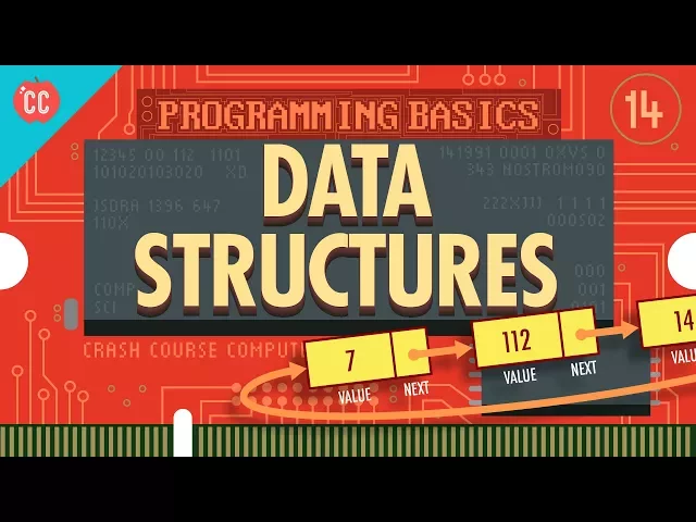
Data Structures: Crash Course Computer Science #14

0:03 Hi, I'm Carrie Anne, and welcome to Crash Course Computer Science!

0:05 Last episode, we discussed a few example classic algorithms,

0:08 like sorting a list of numbers

0:09 and finding the shortest path in a graph.

0:11 What we didn’t talk much about,

0:13 is how the data the algorithms ran on was stored in computer

0:16 memory.

0:16 You don’t want your data to be like John Green’s college dorm room,

0:19 with food, clothing and papers strewn everywhere.

0:21 Instead, we want our data to be structured,

0:23 so that it’s organized, allowing things

0:25 to be easily retrieved and read.

0:27 For this, computer scientists use Data Structures!

0:29 INTRO We already introduced one basic data structure last episode,

0:42 Arrays, also called lists or

0:43 Vectors in some languages.

0:45 These are a series of values stored in memory.

0:47 So instead of just a single value being saved into a variable,

0:50 like ‘j equals 5’, we

0:51 can define a whole series of numbers, and save that into an array variable.

0:55 To be able to find a particular value in this array,

0:58 we have to specify an index.

0:59 Almost all programing languages start arrays at index 0,

1:02 and use a square bracket syntax

1:04 to denote array access.

1:05 So, for example,

1:06 if we want to add the values in the first and third spots of our array

1:10 ‘j’, and save that into a variable ‘a’, we would write a line of code like this.

1:14 How an array is stored in memory is pretty straightforward.

1:16 For simplicity,

1:17 let’s say that the compiler chose to store ours at memory location 1,000.

1:21 The array contains 7 numbers,

1:23 and these are stored one after another in memory, as seen here.

1:26 So when we write “j index of 0”,

1:28 the computer goes to memory location 1,000, with an offset

1:31 of 0, and we get the value 5.

1:33 If we wanted to retrieve “j index of 5”,

1:36 our program goes to memory location 1000,

1:38 plus an offset of 5, which in this case, holds a value of 4.

1:42 It’s easy to confuse the fifth number in the array with the number at index 5.

1:45 They are not the same.

1:46 Remember,

1:46 the number at index 5 is the 6th number in the array because the first number

1:50 is at index 0.

1:51 Arrays are extremely versatile data structures,

1:53 used all the time, and so there are many functions

1:55 that can handle them to do useful things.

1:57 For example,

1:58 pretty much every programming language comes with a built-in sort function,

2:01 where you just pass in your array, and it comes back sorted.

2:04 So there’s no need to write that algorithm from scratch.

2:06 Very closely related are Strings,

2:08 which are just arrays of characters, like letters, numbers,

2:11 punctuation and other written symbols.

2:13 We talked about how computers store characters way back in Episode 4.

2:16 Most often, to save a string into memory, you just put it in quotes, like so.

2:20 Although it doesn’t look like an array, it is.

2:23 Behind the scenes, the memory looks like this.

2:24 Note that the string ends with a zero in memory.

2:27 It’s not the character zero, but the binary value 0.

2:31 This is called the null character, and denotes the end of the string in memory.

2:34 This is important because if I call a function like “print quote”,

2:37 which writes the string

2:38 to the screen,

2:39 it prints out each character in turn starting at the first memory location,

2:42 but it needs to know when to stop!

2:44 Otherwise, it would print out every single thing in memory as text.

2:47 The zero tells string functions when to stop.

2:50 Because computers work with text so often,

2:52 there are many functions that specifically

2:54 handle strings.

2:55 For example,

2:55 many programming languages have a string concatenation function, or “strcat”,

2:59 which takes in two strings, and copies the second one to the end of the first.

3:03 We can use arrays for making one dimensional lists,

3:05 but sometimes you want to manipulate

3:07 data that is two dimensional,

3:08 like a grid of numbers in a spreadsheet, or the pixels

3:11 on your computer screen.

3:12 For this, we need a Matrix.

3:14 You can think of a Matrix as an array of arrays!

3:17 So a 3 by 3 matrix is really 2 an array of size 3,

3:20 with each index storing an array of

3:21 size 3.

3:23 We can initialize a matrix like so.

3:24 In memory, this is packed together in order like this.

3:27 To access a value, you need to specify two indexes,

3:30 like “J index of 2, then index

3:32 of 1”- this tells the computer you’re looking for

3:35 the item in subarray 2 at position 1.

3:37 And this would give us the value 12.

3:39 The cool thing about matrices is we’re not limited

3:40 to 3 by 3— we can make them any

3:42 size we want— and we can also make them any number of dimensions we want.

3:46 For example, we can create a five dimensional matrix and access it like this.

3:50 That’s right,

3:50 you now know how to access a five dimensional matrix— tell your friends!

3:54 So far,

3:55 we’ve been storing individual numbers or letters into our arrays or matrices.

3:59 But often it’s useful to store a block of related variables together.

4:02 Like, you might want to store a bank account number along with its balance.

4:05 Groups of variables like these can be bundled together into a Struct.

4:09 Now we can create variables that aren’t just single numbers,

4:11 but are compound data

4:12 structures, able to store several pieces of data at once.

4:16 We can even make arrays of structs that we define,

4:18 which are automatically bundled together

4:20 in memory.

4:21 If we access, for example, J index of 0,

4:23 we get back the whole struct stored there, and

4:25 we can pull the specific account number and balance data we want.

4:28 This array of structs, like any other array,

4:30 gets created at a fixed size that can’t

4:32 be enlarged to add more items.

4:34 Also, arrays must be stored in order in memory,

4:36 making it hard to add a new item to the middle.

4:38 But, the struct data structure can be used

4:41 for building more complicated data structures

4:42 that avoid these restrictions.

4:44 Let’s take a look at this struct that’s called a “node”.

4:46 It stores a variable, like a number, and also a pointer.

4:49 A pointer is a special variable that points,

4:51 hence the name, to a location in memory.

4:53 Using this struct, we can create a linked list,

4:56 which is a flexible data structure that

4:57 can store many nodes.

4:59 It does this by having each node point to the next node in the list.

5:02 Let’s imagine we have three node structs saved in memory,

5:06 at locations 1000, 1002 and 1008.

5:09 They might be spaced apart,

5:10 because they were created at different times, and other data

5:13 can sit between them.

5:14 So, you see that the first node contains the value 7,

5:17 and the location 1008 in its “next”

5:19 pointer.

5:20 This means that the next node in the

5:22 linked list is located at memory location 1008.

5:24 Looking down the linked list, to the next node,

5:26 we see it stores the value 112 and points

5:28 to another node at location 1002.

5:31 If we follow that,

5:32 we find a node that contains the value 14 and points back to the first

5:36 node at location 1000.

5:37 So this linked list happened to be circular,

5:39 but it could also have been terminated by

5:41 using a next pointer value of 0— the

5:43 null value— which would indicate we’ve reached

5:45 the end of the list.

5:47 When programmers use linked lists,

5:48 they rarely look at the memory values stored in the next

5:50 pointers.

5:51 Instead, they can use an abstraction of a linked list,

5:53 that looks like this, which is

5:55 much easier to conceptualize.

5:56 Unlike an array, whose size has to be pre-defined,

5:59 linked lists can be dynamically extended or

6:01 shortened.

6:02 For example, we can allocate a new node in memory,

6:04 and insert it into this list, just

6:06 by changing the next pointers.

6:07 Linked Lists can also easily be re-ordered, trimmed, split, reversed, and so on.

6:12 Which is pretty nifty!

6:13 And pretty useful for algorithms like sorting, which we talked about last week.

6:16 Owing to this flexibility,

6:17 many more-complex data structures are built on top of linked lists

6:21 The most famous and universal are queues and stacks.

6:23 A queue– like the line at your post office– goes in order of arrival.

6:27 The person who has been waiting the longest, gets served first.

6:30 No matter how frustrating it is that all you want

6:31 to do is buy stamps and the person in

6:33 front of you seems to be mailing 23 packages.

6:36 But, regardless, this behavior is called First-In First-Out, or FIFO.

6:39 That’s the first part.

6:41 Not the 23 packages thing.

6:42 Imagine we have a pointer, named “post office queue”,

6:45 that points to the first node in

6:46 our linked list.

6:47 Once we’re done serving Hank,

6:49 we can read Hank’s next pointer, and update our “post

6:51 office queue” pointer to the next person in the line.

6:54 We’ve successfully dequeued Hank— he’s gone, done, finished.

6:58 If we want to enqueue someone, that is,

6:59 add them to the line, we have to traverse down

7:02 the linked list until we hit the end,

7:03 and then change that next pointer to point to

7:05 the new person.

7:06 With just a small change, we can use linked lists as stacks, which are LIFO…

7:10 Last-In First-Out.

7:11 You can think of this like a stack of pancakes...

7:13 as you make them, you add them to the top

7:15 of stack.

7:16 And when you want to eat one, you take them from the top of the stack.

7:19 Delicious!

7:20 Instead of enqueueing and dequeuing,

7:21 data is pushed onto the stack and popped from the stacks.

7:25 Yep, those are the official terms!

7:27 If we update our node struct to contain not just one,

7:30 but two pointers, we can build trees,

7:32 another data structure that’s used in many algorithms.

7:34 Again, programmers rarely look at the values of these pointers,

7:37 and instead conceptualize trees like this: The top most node is called the root.

7:42 And any nodes that hang from other nodes are called children nodes.

7:45 As you might expect, nodes above children are called parent nodes.

7:48 Does this example imply that Thomas Jefferson is the parent of Aaron Burr?

7:51 I’ll leave that to your fanfiction to decide.

7:54 And finally,

7:54 any nodes that have no children— where the tree ends— are called Leaf Nodes.

7:58 In our example, nodes can have up to two children,

8:01 and for that reason, this particular data

8:03 structure is called a binary tree.

8:04 But you could just as easily have trees with three,

8:07 four or any number of children by modifying

8:09 the data structure accordingly.

8:10 You can even have tree nodes that use linked

8:12 lists to store all the nodes they point to.

8:15 An important property of trees– both in real

8:16 life and in data structures– is that

8:18 there’s a one-way path from roots to leaves.

8:20 It’d be weird if roots connected to leaves, that connected to roots.

8:23 For data that links arbitrarily, that include things like loops,

8:26 we can use a graph data

8:28 structure instead.

8:29 Remember our graph from last episode of cities connected by roads?

8:32 This can be stored as nodes with many pointers,

8:34 very much like a tree, but there is no notion

8:36 of roots and leaves, and children and parents…

8:38 Anything can point to anything!

8:40 So that’s a whirlwind overview of pretty

8:42 much all of the fundamental data structures

8:43 used in computer science.

8:45 On top of these basic building blocks,

8:47 programmers have built all sorts of clever variants, with

8:49 slightly different properties— data structures like red-black trees and heaps,

8:52 which we don’t have time to cover.

8:54 These different data structures have properties

8:56 that are useful for particular computations.

8:59 The right choice of data structure can make your job a lot easier,

9:01 so it pays off to think

9:02 about how you want to structure your data before you jump in.

9:05 Fortunately, most programming languages come with libraries

9:08 packed full of ready-made data structures.

9:10 For example, C++ has its Standard Template Library,

9:13 and Java has the Java Class Library.

9:15 These mean programmers don’t have to

9:17 waste time implementing things from scratch,

9:19 and

9:19 can instead wield the power of data structures to do more interesting things,

9:24 once again allowing us to operate at a new level of abstraction!

9:27 I’ll see you next week.