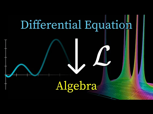
Why Laplace transforms are so useful

0:00 I want to show you this simple simulation that I

0:02 put together that has a mass on a spring,

0:04 but it's being influenced by an external force that oscillates back and forth.

0:09 Now, if there was no external force and you

0:11 pull out this mass and you just let it go,

0:13 the spring has some kind of natural frequency that it wants to oscillate at.

0:17 But here, when I'm adding that external force,

0:19 like a wind blowing back and forth,

0:21 it oscillates at a distinct, unrelated frequency.

0:25 What I want you to notice is how in the beginning,

0:27 you get this very irregular looking behavior.

0:29 It gets kind of stronger, and then weaker,

0:31 and then stronger again, before eventually it settles into a rhythm.

0:35 What specifically is going on there?

0:37 How could you mathematically analyze what exactly this weird,

0:40 wibbly startup trajectory is,

0:42 and could you predict how long it takes before the system hits its stride?

0:46 And when it does hit that stride,

0:48 could you predict exactly how big the swings back and forth are?

0:52 One of the most powerful tools for studying systems like this and many,

0:56 many others is the Laplace transform.

0:58 And today, I want to show you exactly how it looks

1:00 to use this tool to study differential equations and analyze dynamic systems.

1:06 For context, this is the third chapter

1:08 in a sequence all about this Laplace transform.

1:10 And as a very quick recap, in the first chapter,

1:13 you and I became acquainted with functions that look like e to the s times t,

1:17 where s is a complex number,

1:18 and the output of these functions kind of spirals through the complex plane.

1:22 The key concept you have to have

1:24 in your mind is what engineers call the s-plane,

1:27 which is the complex plane representing all possible

1:29 values of this term s in the exponent.

1:33 The idea is to think of each point of the plane

1:36 as encoding the entire function e to the s times t,

1:39 and the primary takeaway is that bigger imaginary

1:42 values of s correspond to functions with more oscillation,

1:45 then negative real parts reflect decay, and positive real parts reflect growth.

1:51 The reason we care is that many functions

1:53 in nature can be broken down into exponential pieces,

1:56 so what we want is a machine that exposes how that breakdown looks.

2:00 This is the key motivation for what Laplace transforms even are,

2:03 and we unpacked that in some detail through the last chapter.

2:07 Again, in the spirit of a quick recap,

2:09 the rough way this transform looks is that it takes

2:12 a function of time and translates it into a new language,

2:15 turning it into a new function whose input is this complex number s.

2:19 The key conclusion from last time is that if

2:22 your function really can be broken into exponential pieces,

2:25 then when you plot this new transformed version over the s-plane,

2:30 poles in that plot correspond to the exponential

2:33 pieces hiding inside the original function.

2:37 Symbolically, this amounts to two key properties that I want you to remember.

2:41 Number one, if you pump in an exponential function,

2:44 something like e to the a times t,

2:47 it transforms into one divided by s minus a, an expression which you should see

2:52 in your mind's eye as a function over the s-plane with a pole above the value a.

2:58 Number two, the transform is linear.

3:01 What this means is if you have a scaled

3:04 sum of functions and then you transform them,

3:06 it's the same as applying the transform to each individual

3:09 function and taking that same scaled sum of the results.

3:13 So for example, if your function going in really

3:15 does look like a combination of exponential terms,

3:18 then what comes out looks like this sum of fractions,

3:21 which you should read in an expression with multiple different poles.

3:25 Each pole reflects one of those exponential pieces.

3:29 These two properties alone already give you a glimpse of why this is

3:33 a helpful tool for getting a qualitative

3:35 sense for the dynamics of some situation.

3:38 If you have some system evolving over time,

3:40 and with techniques I'll show you shortly,

3:42 you're able to find its Laplace transform,

3:44 then when you see poles in this transform with imaginary values,

3:47 that tells you, hey, there's some kind of oscillation.

3:50 If those poles have negative real values,

3:53 that indicates a tendency to decay towards zero,

3:55 but any poles with a positive real part would indicate instability,

3:59 a tendency to explode away from zero.

4:02 Often when you're studying physics,

4:04 you don't know immediately what function describes a dynamic system,

4:07 but you do know a differential equation describing it.

4:11 What's neat is that there's a way to go directly

4:13 from such a differential equation to the Laplace transform of its solution.

4:17 This is useful both as an intermediate step to finding

4:20 an exact solution you can circle on your page, but also equally importantly,

4:25 it's a meaningful representation of the system in its own right.

4:30 The ability to do this is going to rely

4:32 on a third key property that is worth remembering,

4:34 one that explains how exactly Laplace

4:36 transforms can convert differential equations into algebra,

4:39 hence making them easier to solve.

4:42 Here's how it looks.

4:43 If you take the derivative of some function, little f of t,

4:46 with respect to time, and then you take a Laplace transform of that derivative,

4:51 the effect is the same as if you

4:54 had first applied the transform to the original function,

4:57 and then multiplied that result by s, at least almost.

5:01 There's also this additional term where you subtract off the initial condition,

5:05 subtracting the value of your original function,

5:08 little f, at the time t equals zero.

5:11 So in other words, the transform turns differentiation

5:14 in the time domain into multiplication over in the s domain.

5:19 Now, this should feel very reminiscent

5:21 of the fact that, for exponential functions,

5:24 differentiation in time is the same as multiplication by s,

5:27 and it's no coincidence that ultimately the underlying reason is the same.

5:32 Now, at first glance, when you look at this rule,

5:35 that little minus f of zero term might seem like

5:37 kind of an annoying quirk to an otherwise very elegant equation,

5:40 but really it's a feature, not a bug.

5:42 As you apply this to differential equations, this little quirk means you have

5:46 a built-in way to account for initial conditions.

5:49 Now, I can hear you asking, why is this property true?

5:52 Where does it come from?

5:54 How exactly is this connected to the idea of differentiating an exponential,

5:58 and where does that minus f of zero term come from in the first place?

6:02 I will, of course, explain this.

6:04 In fact, I can think of three ways to explain it,

6:06 but let's postpone those for just a minute and instead

6:09 dive into how you actually use this property in practice.

6:13 The example I want to show starts with the simple harmonic oscillator,

6:16 which is something you and I studied two chapters

6:18 ago where you might imagine a mass on a spring.

6:21 As a reminder, one component of the force that acts on that mass pulls it

6:25 towards a middle position with a strength that's

6:28 proportional to its distance away from that middle.

6:31 We write that as negative k times x.

6:34 And it's also common to include a damping force,

6:36 which acts by slowing down this mass's

6:39 movement with a strength proportional to its velocity,

6:42 again using some negative proportionality constant.

6:46 And then the algebra always ends up looking very nice if we move

6:49 all of these terms to just one side of the equation, like this.

6:52 With no further modification,

6:53 this right here is a very friendly linear equation.

6:56 We talked all about how to solve it simply by substituting in e to the st,

7:01 which, depending on your perspective,

7:03 is either a frustratingly unmotivated guess,

7:05 or that's just the established procedure you do once you've learned

7:09 the fundamental fact that linear equations

7:11 like this always have an exponential solution.

7:15 That's all previous material,

7:16 but this time we're going to imagine there is a third force acting on the mass,

7:21 some kind of external force, which in our example will oscillate back

7:25 and forth according to a cosine function,

7:27 like a wind with periodic gusts to the left and to the right.

7:31 Importantly, the frequency of this external force will generally have

7:34 nothing to do with the natural resonant frequency for the spring.

7:38 And this is not an arbitrary example that came up for us before

7:41 on this channel when we studied why light slows down in a medium like glass.

7:45 In that context, once we were deep into the video,

7:48 the relevant oscillator was a little charge inside the material,

7:52 and the external force was an incoming light wave.

7:55 Faced with an equation like this, which is no longer a linear equation,

7:59 it's more complicated to solve, here's a preview of the general strategy.

8:03 What you do is you take a Laplace transform of all of the terms,

8:06 and then you can solve that result

8:08 to reveal the transformed version of the solution,

8:11 and then from there you can invert the process

8:14 to recover that solution in our usual language,

8:16 in the time domain instead of the s domain.

8:19 Okay, that's the high-level view,

8:20 but let's roll up our sleeves and actually step through this piece by piece.

8:24 Following the usual convention,

8:26 I'm going to write the transform for little x of t as capital X of s,

8:31 and then using the rule that we just talked all about,

8:33 the transform for its derivative is going to look like s times capital X,

8:38 all minus an initial condition, which I'm going to write as little x naught.

8:43 And then for the second derivative, what should that look like?

8:46 This is actually a good chance to pause and try it out as an exercise.

8:49 It basically looks like applying that key rule

8:51 we just talked about, but twice in a row.

8:53 Applying it once, you get that the transform of the second

8:57 derivative should look like s times the transform of the first derivative,

9:00 all minus x prime of zero.

9:02 That term is the same as the initial velocity, so I'll write it as v naught.

9:06 This is where, in the whole procedure,

9:08 that part of the initial condition is kind of automatically accounted for.

9:12 And from here, you can substitute

9:14 in the Laplace transform of that derivative as, again,

9:17 s times capital X of s, all minus an initial condition.

9:20 We can distribute a couple terms here, substitute it back up in what we had,

9:24 and if we bring along those other constants, m, mu, and k for the ride,

9:28 we get this kind of large but not wholly unreasonable expression.

9:32 And what I want to draw your attention to are these three terms here,

9:36 the ones that include a component of capital X of s.

9:40 If we add those together and factor out the whole capital X part,

9:43 what we're left with is a nice little quadratic polynomial.

9:47 What would be very clean and pretty is if that's all we had,

9:50 but messing up the elegance is that we have

9:52 all of these initial condition terms kind of riding along.

9:55 And I say they're messing up the elegance,

9:57 but again I want to point out it actually is

9:59 very nice to have a baked-in way to incorporate initial conditions,

10:01 that's not going to be some added step later on.

10:04 Nevertheless, for the sake of a clean initial example,

10:07 let's assume that both the initial position and the initial velocity are zero,

10:11 so our spring on a mass starts off completely stationary.

10:15 Keep in mind, for a more general solution,

10:17 you might want to keep these constants around.

10:19 What's nice about ignoring them is that it shines

10:22 a light on a characteristic pattern of applying Laplace transforms,

10:25 where this part of our differential equation, the left-hand side on the top,

10:30 basically gets turned into a polynomial that looks

10:32 like a kind of mirror image of it, one that has all the same constants,

10:36 and where each higher-order derivative, like that x double prime,

10:40 turns into some power of s, in this case s squared.

10:43 That is really the essence of why this tool works.

10:46 Differential expressions turn into polynomials,

10:48 and polynomials are something we can do algebra with.

10:50 But of course, for this example, what makes it interesting is that we have

10:54 this other oscillating force on the right-hand side,

10:57 and taking a Laplace transform of a cosine expression

10:59 is something we talked all about in the previous episode.

11:03 In practice, this is the kind of thing

11:05 you would either have memorized or look up, but if you want to pause,

11:09 I think this is a good chance for an exercise to take a moment and see

11:12 if you remember why the transform

11:14 of a cosine expression should have two different poles,

11:17 in this case one pole at omega i, and the other pole at negative omega i,

11:21 and take a moment to quickly gut check

11:23 that that lines up with the expression you're looking at here,

11:26 with this denominator s squared plus omega squared.

11:29 What I really want to pop into your mind's eye when you see

11:33 that in the denominator is the idea of poles at omega i and omega negative i,

11:37 and with a nice intuition of the s-plane,

11:39 that should feel in your bones like oscillation with a frequency of omega.

11:44 The next step when it comes to just pushing around the symbols

11:47 on the page is to divide out by this component here.

11:50 And with that, you now have an exact final expression, fully describing,

11:54 well not the solution of your system, but the Laplace transform of its solution.

11:59 As I previewed, the final step will be to invert the Laplace transform process,

12:03 revealing the original mystery function,

12:05 but before that, even just at this step,

12:07 I want you to notice how by seeing this transformed version,

12:10 you already get a lot of intuition for the dynamics of the system.

12:14 Remember, the key question over in the s domain is where are all the poles,

12:19 and this expression has a pole wherever its denominator is equal to zero.

12:24 In this example, there are four different

12:26 values of s that make this denominator zero.

12:29 Two of them come from the roots of this polynomial here,

12:32 the one I described as a mirror image of the harmonic oscillator equation.

12:37 Any of you who watched the previous chapters will remember how this looks.

12:40 It amounts to applying the quadratic formula, and as you tweak the constants k,

12:45 mu, and m, the roots of that polynomial fall in different places on the S-plane.

12:51 But generally, they have a negative real part,

12:53 and, assuming the damping coefficient is not too big,

12:56 they have an imaginary part.

12:58 And when you see points on the S-plane like that, what should pop

13:01 into your mind's eye is the notion of oscillation with some kind of decay.

13:05 In other words, even when you add this external force to the oscillator,

13:10 the solution of the unforced oscillator,

13:12 what it would do on its own, is still lurking inside.

13:16 Hidden somewhere in there is the oscillation matching

13:18 the natural resonant frequency of the spring system.

13:21 The other poles of our transformed function come

13:24 from the roots of this part right here, which are omega i and negative omega i,

13:29 and those correspond to the cosine external force.

13:32 In other words, another component of the final dynamics,

13:36 really the dominant component in this case,

13:38 is a tendency to oscillate in sync with that external force.

13:43 And this should feel intuitive.

13:44 If you go and push a kid on a swing,

13:47 but with a frequency that doesn't necessarily

13:48 match the natural resonant frequency of the swing,

13:51 what ultimately happens to their motion is that they

13:54 also oscillate in a way that matches your frequency,

13:57 not the natural one of the swring.

14:00 Here, this might all make a little bit more

14:02 sense if I return back to that simulation that I

14:04 opened with, that has a graph on the top showing

14:07 the position of this mass on a spring over time.

14:10 Again, notice how that graph has this weird initial startup

14:13 period where it's sort of wibbling about finding its stride,

14:16 but eventually it does fall into that rhythm

14:18 and follow this consistent sine wave pattern, synced up with the external force.

14:23 What's going on here is that the solution can

14:25 be thought of as a sum of two different components.

14:29 One component corresponds to those poles on the left half of the S-plane,

14:33 and it matches a solution to the unforced equation,

14:37 what the spring would do without any external influence.

14:41 The other component corresponds to the two poles

14:44 of the Laplace transform on the imaginary axis,

14:47 meaning it's pure oscillation with no growth or decay,

14:50 and it's simply a cosine wave matching the rhythm of that external force.

14:54 From this perspective,

14:56 you can recognize how that initial period of wibbling about

14:59 corresponds to the time when that first component is still relevant.

15:03 You have these two distinct frequencies competing with each other,

15:07 and that first one has not yet decayed away into obscurity,

15:10 but eventually it does, leaving behind only the pure cosine.

15:15 Okay, okay, okay, I hear some of you saying,

15:17 that's all well and good, but what is the actual solution?

15:20 I have an exam tomorrow,

15:21 and I need to circle some expression at the bottom of my paper.

15:24 Well, if you do want an exact analytic solution,

15:27 this next part is not exactly fun, but it is straightforward.

15:31 If you have a fraction like this one that we found,

15:34 and you know the roots of its denominator,

15:37 like the four roots that we just discussed,

15:39 you can break it up as a sum of four fractions where

15:42 the denominator of each one looks like s minus one of those roots.

15:46 The work you have to do goes

15:48 into solving for these constants up in the numerator.

15:50 There's a process for it, it's called partial fraction decomposition.

15:53 I'm not going to walk through the details,

15:55 I don't think you want me to walk through the details,

15:57 but I'll leave up the key idea as a little on-screen note.

16:01 Once you do solve for those constants,

16:03 because you know that an exponential term transforms into a simple fraction,

16:06 like the ones we're looking at, inverting

16:09 the process amounts to inverting that one key rule.

16:12 You turn each of these fractions into the appropriate exponential term.

16:16 So the locations of each pole, those roots of the denominator,

16:19 correspond to the values in the exponents sitting in front of the time t.

16:24 And those constants that you have to put in the work to solve

16:27 for remain as the constants in front of each of these exponentials.

16:31 If you're the kind of person who

16:33 likes homework and enjoys digging into the formulas,

16:35 and you choose to take on the challenge of solving for those constants,

16:38 there's one very interesting conclusion of that exercise I want you to focus on.

16:42 Look at the first two terms, corresponding to the poles +ωi and -ωi.

16:47 When you solve for the two relevant constants,

16:49 the expressions you get are not quite the same, but if mu is very close to zero,

16:54 each one is approximately this shared expression that we can factor out.

16:59 Now, you know that two imaginary exponentials

17:02 like this combine to make a cosine.

17:04 So this part you're looking at is that final

17:07 steady-state cosine rhythm that the mass eventually falls into.

17:10 And inside that big expression that you solve for, the exercise I

17:14 want to leave you with as homework is to think deeply about

17:17 how the amplitude of this final expression depends on the difference between

17:22 the resonant frequency of the spring and the frequency of that external force.

17:27 In particular, what happens as both of those frequencies get closer together?

17:32 And how might this be relevant to anyone wishing to build

17:34 a bridge that they don't want to wobble into ruin?

17:39 Stepping out from the trees to look over the forest,

17:42 you see what I mean about how Laplace

17:44 transforms can turn a differential equation into algebra,

17:47 and how it's all rooted in this third key property

17:50 where a derivative in time turns into multiplication by s.

17:54 So naturally, the burning question is,

17:55 why is this property true in the first place?

17:58 And like I said, I can think of three different ways to explain it.

18:01 One that's elementary but limited, one that's general but a bit opaque,

18:05 and then there's my favorite, which requires a little added theory to describe.

18:10 The first one is actually not a complete explanation.

18:13 The idea is that any time you see a new formula in math,

18:16 it's never a bad idea to just try it out on an example you know well.

18:20 That way you build a little intuition.

18:22 In this case, what's an example that you and I know very well?

18:26 Well, we have emphasized to death the fact

18:28 that if you pump in an exponential function, something like e to the a t,

18:33 then its Laplace transform looks like 1 divided by s minus a.

18:36 So let's see what happens for this example.

18:39 You know how to take the derivative of an exponential like this.

18:42 It's delightfully simple, you just multiply by that constant a.

18:45 And then, because of linearity,

18:47 this means the Laplace transform also just picks up that added factor of a.

18:52 And at first, this actually seems wrong.

18:54 It seems inconsistent with the desired conclusion.

18:58 We're not multiplying by s, the input of our new transformed function.

19:02 Instead, the thing we're multiplying by is this random constant

19:05 a that characterizes what specific exponential we happened to throw in.

19:09 But this is really just a matter of some gentle algebraic massaging.

19:13 Notice what happens if I add this fraction,

19:15 s minus a over s minus a, which is the same as adding 1,

19:19 so I have to subtract off 1 to account for it.

19:22 When you combine these two fractions here,

19:24 you get some nice cancellation in the numerator,

19:26 leaving behind this clean factor of s.

19:29 And you'll notice we're now subtracting

19:31 off something from the whole expression, 1.

19:33 And that happens to be the initial condition.

19:36 It's what you get if you plug in t

19:38 equals 0 to the original function we pumped in.

19:41 So in fact, it really is consistent with the desired conclusion.

19:45 Now of course, this is just one very specific function,

19:48 this is not a general explanation,

19:49 but it holds within it the seeds of much more generality.

19:53 If you like exercises, take a moment to convince yourself that this result

19:57 is also true for any combination of exponential functions.

20:01 This really just amounts to leaning hard on linearity again,

20:05 both linearity of the transform and of the derivative.

20:08 This is still not a complete explanation,

20:10 it only applies to combinations of exponentials,

20:13 but to be fair that includes every example we've seen so far,

20:16 and an overarching theme of this whole series will be how many,

20:19 many things really can be broken into exponentials with the right point of view.

20:25 The second explanation I want to at least briefly flash

20:27 up here is the one that you'll see in most textbooks.

20:30 The idea is to simply pull up the definition of a Laplace transform,

20:33 which somewhat bizarrely we actually haven't had

20:35 to look at ever since the last chapter,

20:38 and then to evaluate it, you apply integration by parts.

20:41 This is another case where I think it's best to just leave the details

20:44 on screen for any curious and calculus-savvy students

20:46 who want to pause and think it through.

20:49 It's a perfectly fine and tidy derivation, really short actually,

20:52 but sometimes I feel like whenever you appeal to integration by parts,

20:56 you can almost see the intuition evaporating

20:58 away from the audience in front of you.

21:01 And in this case, if you stop and ask yourself where

21:04 that times s really came from, or why we're subtracting an initial condition,

21:09 both of them kind of feel like things that happened to fall out.

21:13 The third explanation, at least in my own head,

21:15 is what really shows why the property is not just true,

21:19 but woven into the fabric of what a Laplace transform was born to do.

21:23 The caveat is that it requires

21:25 understanding something we haven't talked about yet,

21:27 known as the inverse Laplace transform.

21:30 This is something you might have already started wondering about.

21:32 If you look back at our differential equation example,

21:35 in that very last step where we

21:37 inverted the process to recover the original function,

21:40 a perfectly reasonable question to ask would be how is this supposed

21:43 to work if you can't necessarily break

21:45 the result into these clean fractional pieces?

21:48 That question is very closely tied to the question

21:51 of what Laplace transforms mean if your original

21:54 function cannot be broken down into a discrete

21:56 sum of exponential pieces in the first place.

22:00 This inverse transform is a big enough topic that it deserves its own chapter.

22:04 For example, it involves a fun new concept for us known as a contour integral.

22:09 What I'd like to do with that next chapter is

22:12 walk through how you could reinvent this tool for yourself,

22:15 starting from a desire to create something that has this third key

22:18 property we've been focusing on, where

22:21 derivatives turn into a kind of multiplication.

22:24 I think there's a very natural storyline

22:26 where slowly tugging on a certain logical thread

22:29 leads you to inventing both the Laplace transform

22:31 and its inversion formula as a unified pair.

22:35 Along the way, you also get to see

22:36 how it relates to Fourier transforms and Fourier inversion.

22:40 If you're feeling up for a jaunt into the deeper theory of the subject,

22:43 come join me in the next chapter.