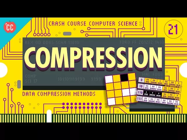
Compression: Crash Course Computer Science #21
CrashCourse
0:03 This episode is brought to you by Curiosity Stream.
0:05 Hi, I'm Carrie Anne, and welcome to Crash Course Computer Science!
0:09 Last episode we talked about Files, bundles of data, stored on a computer,
0:12 that are formatted and arranged to encode information,
0:15 like text, sound or images.
0:17 We even discussed some basic file formats, like text, wave, and bitmap.
0:20 While these formats are perfectly fine and still used today,
0:23 their simplicity also means they’re not very efficient.
0:26 Ideally, we want files to be as small as possible,
0:28 so we can store lots of them without filling up our hard drives,
0:31 and also transmit them more quickly.
0:33 Nothing is more frustrating than waiting for an email attachment to download.
0:36 Ugh!
0:37 The answer is compression, which literally squeezes data into a smaller size.
0:41 To do this, we have to encode
0:43 data using fewer bits than the original representation.
0:46 That might sound like magic, but it’s actually computer science!
0:49 INTRO Lets return to our old friend from last episode, Mr.
1:01 Pac-man!
1:01 This image is 4 pixels by 4 pixels.
1:04 As we discussed, image data is typically stored as a list of pixel values.
1:08 To know where rows end,
1:09 image files have metadata, which defines properties like dimensions.
1:12 But, to keep it simple today, we’re not going to worry about it.
1:15 Each pixel’s color is a combination of three additive primary colors:
1:19 red, green and blue.
1:20 We store each of those values in one byte,
1:23 giving us a range of 0 to 255 for each color.
1:26 If you mix full intensity red,
1:27 green and blue- that’s 255 for all three values- you get the color white.
1:32 If you mix full intensity red and green, but no blue (it’s 0), you get yellow.
1:36 We have 16 pixels in our image, and each of those needs 3 bytes of color data.
1:41 That means this image’s data will consume 48 bytes of storage.
1:44 But, we can compress the data and pack
1:46 it into a smaller number of bytes than 48!
1:48 One way to compress data is to reduce repeated or redundant information.
1:52 The most straightforward way to do this is called Run-Length Encoding.
1:55 This takes advantage of the fact that there
1:57 are often runs of identical values in files.
1:59 For example, in our pac-man image, there are 7 yellow pixels in a row.
2:03 Instead of encoding redundant data: yellow pixel, yellow pixel, yellow pixel,
2:06 and so on, we can just say “there’s 7 yellow pixels in a row”
2:10 by inserting an extra byte that specifies the length of the run,
2:14 like so: And then we can eliminate the redundant data behind it.
2:17 To ensure that computers don’t get confused with which
2:19 bytes are run lengths and which bytes represent color,
2:22 we have to be consistent in how we apply this scheme.
2:25 So, we need to preface all pixels with their run-length.
2:28 In some cases, this actually adds data, but on the whole,
2:31 we’ve dramatically reduced the number of bytes we need to encode this image.
2:34 We’re now at 24 bytes, down from 48.
2:37 That’s 50% smaller!
2:38 A huge saving!
2:40 Also note that we haven’t lost any data.
2:42 We can easily expand this back to the original form without any degradation.
2:45 A compression technique that has
2:47 this characteristic is called lossless compression,
2:49 because we don’t lose anything.
2:51 The decompressed data is identical
2:53 to the original before compression, bit for bit.
2:56 Let's take a look at another type of lossless compression,
2:58 where blocks of data are replaced by more compact representations.
3:02 This is sort of like “don’t forget to be awesome” being replaced by DFTBA.
3:06 To do this, we need a dictionary that stores the mapping from codes to data.
3:10 Lets see how this works for our example.
3:12 We can view our image as not just a string of individual pixels,
3:15 but as little blocks of data.
3:16 For simplicity, we’re going to use pixel pairs,
3:18 which are 6 bytes long, but blocks can be any size.
3:22 In our example, there are only four pairings:
3:25 White-yellow, black-yellow, yellow-yellow and white-white.
3:27 Those are the data blocks in our dictionary
3:29 we want to generate compact codes for.
3:31 What’s interesting, is that these blocks occur at different frequencies.
3:34 There are 4 yellow-yellow pairs, 2 white-yellow pairs,
3:37 and 1 each of black-yellow and white-white.
3:39 Because yellow-yellow is the most common block,
3:41 we want that to be substituted for the most compact representation.
3:45 On the other hand, black-yellow and white-white,
3:47 can be substituted for something longer because those blocks are infrequent.
3:51 One method for generating efficient codes is building a Huffman Tree,
3:54 invented by David Huffman while he was a student at MIT in the 1950s.
3:58 His algorithm goes like this.
4:00 First, you layout all the possible blocks and their frequencies.
4:03 At every round, you select the two with the lowest frequencies.
4:05 Here, that’s Black-Yellow and White-White, each with a frequency of 1.
4:10 You combine these into a little tree...
4:11 ...which have a combined frequency of 2, so we record that.
4:15 And now one step of the algorithm done.
4:17 Now we repeat the process.
4:18 This time we have three things to choose from.
4:20 Just like before, we select the two with the lowest frequency,
4:23 put them into a little tree,
4:25 and record the new total frequency of all the sub items.
4:27 Ok, we’re almost done.
4:29 This time it’s easy to select the two items with the lowest
4:32 frequency because there are only two things left to pick.
4:34 We combine these into a tree, and now we’re done!
4:37 Our tree looks like this, and it has a very cool property:
4:40 it’s arranged by frequency, with less common items lower down.
4:43 So, now we have a tree,
4:44 but you may be wondering how this gets us to a dictionary.
4:46 Well, we use our frequency-sorted tree to generate the codes we
4:50 need by labeling each branch with a 0 or a 1,
4:53 like so: With this, we can write out our code dictionary.
4:56 Yellow-yellow is encoded as just a single 0.
4:59 White-yellow is encoded as 1 0 (“one zero”) Black-Yellow is
5:01 1 1 0 and finally white-white is 1 1 1.
5:04 The really cool thing about these codewords is
5:06 that there’s no way to have conflicting codes,
5:08 because each path down the tree is unique.
5:10 This means our codes are prefix-free,
5:12 that is no code starts with another complete code.
5:15 Now, let’s return to our image data and compress it!
5:18 Our first pixel pair, white-yellow, is substituted for the bits “1 0”.
5:21 The next pair is black-yellow, which is substituted for “1 1 0”.
5:25 Next is yellow-yellow with the incredibly compact substitution of just “0”.
5:29 And this process repeats for the rest of the image:
5:32 So instead of 48 bytes of image data ...this process
5:34 has encoded it into 14 bits— NOT BYTES— BITS!!
5:38 That’s less than 2 bytes of data!
5:40 But, don’t break out the champagne quite yet!
5:42 This data is meaningless unless we also save our code dictionary.
5:45 So, we’ll need to append it to the front of the image data, like this.
5:49 Now, including the dictionary, our image data is 30 bytes long.
5:53 That’s still a significant improvement over 48 bytes.
5:56 The two approaches we discussed, removing redundancies and using more
5:59 compact representations, are often combined,
6:01 and underlie almost all lossless compressed file formats,
6:04 like GIF, PNG, PDF and ZIP files.
6:07 Both run-length encoding and dictionary
6:09 coders are lossless compression techniques.
6:11 No information is lost; when you decompress, you get the original file.
6:14 That’s really important for many types of files.
6:17 Like, it’d be very odd if I zipped up a word document to send to you,
6:20 and when you decompressed it on your computer, the text was different.
6:23 But, there are other types of files where we can get away with little changes,
6:26 perhaps by removing unnecessary or less important information,
6:29 especially information that human perception is not good at detecting.
6:33 And this trick underlies most lossy compression techniques.
6:37 These tend to be pretty complicated,
6:38 so we’re going to attack this at a conceptual level.
6:41 Let’s take sound as an example.
6:42 Your hearing is not perfect.
6:44 We can hear some frequencies of sound better than others.
6:47 And there are some we can’t hear at all, like ultrasound.
6:49 Unless you’re a bat.
6:50 Basically, if we make a recording of music,
6:52 and there’s data in the ultrasonic frequency range,
6:54 we can discard it, because we know that humans can’t hear it.
6:58 On the other hand, humans are very sensitive to frequencies in the vocal range,
7:01 like people singing, so it’s best to preserve quality there as much as possible.
7:05 Deep bass is somewhere in between.
7:07 Humans can hear it, but we’re less attuned to it.
7:09 We mostly sense it.
7:11 Lossy audio compressors takes advantage of this, and encode
7:13 different frequency bands at different precisions.
7:16 Even if the result is rougher,
7:18 it’s likely that users won’t perceive the difference.
7:20 Or at least it doesn’t dramatically affect the experience.
7:23 And here comes the hate mail from the audiophiles!
7:25 You encounter this type of audio compression all the time.
7:28 It’s one of the reasons you sound different on a cellphone versus in person.
7:32 The audio data is being compressed, allowing more people to take calls at once.
7:35 As the signal quality or bandwidth get worse,
7:38 compression algorithms remove more data, further reducing precision,
7:41 which is why Skype calls sometimes sound like robots talking.
7:44 Compared to an uncompressed audio format, like a WAV or FLAC (there we go,
7:48 got the audiophiles back) compressed audio files,
7:50 like MP3s, are often 10 times smaller.
7:53 That’s a huge saving!
7:55 And it’s why I’ve got a killer music collection on my retro iPod.
7:58 Don’t judge.
7:59 This idea of discarding or reducing precision in a manner
8:01 that aligns with human perception is called perceptual coding,
8:04 and it relies on models of human perception,
8:07 which come from a field of study called Psychophysics.
8:09 This same idea is the basis of lossy compressed image formats,
8:13 most famously JPEGs.
8:14 Like hearing, the human visual system is imperfect.
8:16 We’re really good at detecting sharp contrasts, like the edges of objects,
8:20 but our perceptual system isn’t so hot with subtle color variations.
8:23 JPEG takes advantage of this by breaking images up into blocks of 8x8 pixels,
8:28 then throwing away a lot of the high-frequency spatial data.
8:31 For example, take this photo of our directors dog- Noodle.
8:33 So cute!
8:34 Let’s look at patch of 8x8 pixels.
8:37 Pretty much every pixel is different from its neighbor,
8:39 making it hard to compress with loss-less
8:41 techniques because there’s just a lot going on.
8:43 Lots of little details.
8:45 But human perception doesn’t register all those details.
8:47 So, we can discard a lot of that detail,
8:49 and replace it with a simplified patch like this.
8:52 This maintains the visual essence, but might only use 10% of the data.
8:55 We can do this for all the patches in the image and get this result.
8:58 You can still see it’s a dog, but the image is rougher.
9:01 So, that’s an extreme example,
9:02 going from a slightly compressed JPEG to a highly compressed one,
9:05 one-eighth the original file size.
9:07 Often, you can get away with a quality somewhere in between,
9:11 and perceptually, it’s basically the same as the original.
9:13 The one on the left is one-third the file size of the one on the right.
9:16 That’s a big savings for essentially the same thing.
9:19 Can you tell the difference between the two?
9:21 Probably not, but I should mention that video
9:23 compression plays a role in that too,
9:25 since I’m literally being compressed in a video right now.
9:27 Videos are really just long sequences of images,
9:28 so a lot of what I said about them applies here too.
9:32 But videos can do some extra clever stuff, because between frames,
9:34 a lot of pixels are going to be the same.
9:37 Like this whole background behind me!
9:39 This is called temporal redundancy.
9:41 We don’t need to re-transmit those pixels every frame of the video.
9:44 We can just copy patches of data forward.
9:46 When there are small pixel differences,
9:48 like the readout on this frequency generator behind me,
9:51 most video formats send data that encodes just the difference between patches,
9:54 which is more efficient than re-transmitting all the pixels afresh,
9:58 again taking advantage of inter-frame similarity.
10:01 The fanciest video compression formats go one step further.
10:04 They find patches that are similar between frames,
10:06 and not only copy them forward,
10:08 with or without differences, but also can apply simple effects to them,
10:11 like a shift or rotation.
10:13 They can also lighten or darken a patch between frames.
10:16 So, if I move my hand side to side
10:18 like this the video compressor will identify the similarity,
10:21 capture my hand in one or more patches,
10:23 then just move these patches around between frames.
10:25 You’re actually seeing my hand from the past… kinda freaky,
10:28 but it uses a lot less data.
10:30 MPEG-4 videos, a common standard,
10:31 are often 20 to 200 times smaller than the original, uncompressed file.
10:35 However, encoding frames as translations and rotations of patches from previous
10:40 frames can go horribly wrong when you compress too heavily,
10:42 and there isn’t enough space to update pixel data inside of the patches.
10:46 The video player will forge ahead, applying the right motions,
10:49 even if the patch data is wrong.
10:51 And this leads to some hilarious and trippy effects, which I’m sure you’ve seen.
10:54 Overall, it’s extremely useful to have compression techniques
10:56 for all the types of data I discussed today.
10:59 (I guess our imperfect vision and hearing are “useful,” too.) And it’s
11:02 important to know about compression because it allows users to store pictures,
11:05 music, and videos in efficient ways.
11:07 Without it, streaming your favorite Carpool Karaoke
11:09 videos on YouTube would be nearly impossible,
11:12 due to bandwidth and the economics of transmitting that volume of data for free.
11:17 And now when your Skype calls sound like they’re being taken over by demons,
11:20 you’ll know what’s really going on.
11:21 I’ll see you next week.
11:23 Hey guys, this week’s episode was brought to you by CuriosityStream which is
11:26 a streaming service full of documentaries
11:28 and nonfiction titles from some really great filmmakers,
11:31 including exclusive originals.
11:33 Now I normally give computer science recommendations since this is Crash Course
11:37 Computer Science and all and Curiosity Stream has a ton of great ones.
11:41 But you absolutely have to check out “Miniverse” starring everyone’s favorite
11:46 space-station-singing-Canadian astronaut, Chris Hadfield,
11:47 as he takes a roadtrip across the Solar System
11:50 scaled down the the size of the United States.
11:53 It’s basically 50 minutes of Chris and his passengers geeking out
11:56 about our amazing planetary neighbors and you don’t want to miss it.
12:00 So get unlimited access today, and your first two months are free if you sign up
12:06 at curiositystream.com/crashcourse and use the promo
12:08 code "crashcourse" during the sign up process.