Generating Performant 6G GPU-Accelerated Code From High-Level Programming Languages

0:00 Okay, thank you Emeka.

0:01 So this is a follow-up talk to Michael's

0:03 great talk on the Aerial Framework runtime.

0:06 So before I get started, just to remind people that this is available

0:11 on GitHub and we have the getting started tutorials.

0:15 Michael covered 1, 7, 8, and 9.

0:18 And in this talk I'm going to cover the middle tutorials

0:22 on Python and how to take Python down to performant GPU code.

0:27 So as Michael said the Aerial Framework has two environments.

0:31 This is the development environment

0:33 with the lowering toolchain and the runtime engine.

0:36 The runtime engine has the GPU plus a NIC and this is

0:40 needed to run the real-time applications with MAC and radio unit emulation.

0:45 And this is really built for your test beds and product.

0:48 Now the development is the part that I'll talk about now.

0:52 And this is available to anyone with a recent GPU,

0:57 and it's for compiling algorithms to GPU executable code

1:00 for the Aerial Framework runtime engine over here or for test

1:04 beds if you have your own GPU C++ pipeline

1:09 product trials or if you have a C++ simulator.

1:13 So radio access networks have been well studied for decades

1:17 and we understand them very well in simulations and theory.

1:21 But the real world is messy.

1:24 Wireless radio channels don't really capture—I mean the 3GPP

1:28 models don't really capture—the true richness of the world

1:31 and data traffic patterns that we use in 3GPP

1:35 standardization don't represent modern apps and generative AI data flows.

1:38 And of course in the real

1:40 world we have hardware imperfections and nonlinearities.

1:43 And many may not know this but UE implementations,

1:47 the actual mobile phones, they differ from one another.

1:51 So in practice there are lots of heuristics, assumptions,

1:55 and compromises that are used to get things working.

1:59 So we believe that AI will help drive the next innovation wave.

2:03 And later in the talk I'm going to dig deep

2:06 into an example where we have a classical channel estimator fused with AI.

2:11 Okay.

2:12 So, we're going to use a transformer inside the channel estimator to basically

2:18 predict the parameters of the channel filter

2:22 using that channel estimator to improve performance.

2:25 So, in a world where we have signal processing deeply fused with AI,

2:30 how do we take this type of code to product?

2:33 How do we make it run real time over the air?

2:37 And this is where the Aerial Framework comes in.

2:40 So to explain this idea, I'd like to use this graph.

2:44 So on the x-axis we have runtime latency.

2:47 So this is in milliseconds.

2:49 This line here indicates the magic one slot marker of 500 microseconds.

2:55 Over here this is slower.

2:57 This would be milliseconds or seconds.

3:00 And over here fast that we need for the over-the-air transmission.

3:05 On the y-axis we have the iteration speed of how quickly or how

3:10 easy it is to innovate your algorithms and AI to improve system performance.

3:14 So the top fast few days and at the bottom slow where it takes years.

3:21 So first up research simulators.

3:23 These are typically written in Python and MATLAB

3:25 because you need to iterate your ideas fast.

3:28 You need to prototype.

3:30 You need native integration of Torch and JAX to use AI.

3:35 And as far as I know,

3:37 there is no one simulator that covers the entire RAN stack.

3:40 Like, the RAN stack is just too complicated.

3:43 So, everyone has their own simulator that simulates a part of the stack.

3:48 So, the next up in the pipeline is test beds.

3:51 And this is where you take ideas from simulators

3:54 and you rewrite the algorithms in C++ or CUDA

3:58 to get performance that you need to go

4:00 over the air within this 500 microsecond slot time.

4:05 And finally we have the product implementations and this is

4:10 where you have extreme optimizations in C++ and CUDA

4:14 to get ultra low latencies for large workloads where you

4:19 have SLAs and very rigid uptime requirements for real world deployments.

4:26 So how does an idea go from research to test bed to product?

4:30 The way I like to think about it is we have researchers.

4:34 They come up with the algorithm and then they write what is like a paper IR,

4:39 a paper intermediate representation,

4:40 where they write the algorithm down on paper or in a PowerPoint slide and it

4:44 gets handed over to someone who implements

4:46 a more serious version for a test or product.

4:50 But what I find is when we get down to these ultra

4:56 optimized implementations that lots of the nuance around the algorithm

4:59 and why it was designed that way have been lost

5:02 and the algorithm and the platform becomes incredibly fixed and rigid.

5:06 So it becomes very slow to integrate new ideas and test out things.

5:11 So the Aerial runtime engine that Michael introduced has been built

5:16 on years of learnings from Aerial and GPU teams and it's

5:20 really built for product and test bed workloads and they

5:23 have done a wonderful job at separating between runtime and algorithms.

5:28 So the question is how do we use this now

5:32 to accelerate research and this is the point of the Aerial Framework,

5:37 is to take research code directly from Python and push it into test

5:42 beds where you can verify it where it matters and that's over the air.

5:48 So the vision is to connect research, test beds,

5:51 and product to help solve development challenges at real time and by real time

5:55 I mean microsecond latency applications and then

5:57 we want developers to develop on C’s hardware,

6:00 for example DGX Spark or an RTX graphics card,

6:03 and then take the same code and deploy it

6:07 to product to test their ideas for real over the air.

6:11 So we want our software developers to have

6:13 state-of-the-art tools for signal processing and AI.

6:16 We very much don't want RAN software development

6:19 to get left behind other areas like AI,

6:22 automotive, robotics and scientific computing.

6:24 So this is the point of the Aerial Framework.

6:28 So we built this for RAN engineers and researchers

6:30 and I thought I'd go through two workflow examples,

6:33 and starting off with a very simple finite impulse response filter.

6:38 So here we have the equation defining the filter.

6:42 X is the input sequence.

6:44 In the figure here, it's this gray line, very noisy gray line.

6:48 And we want to filter it with this kernel H.

6:51 And we filter by sliding the kernel H

6:54 over the sequence in time and computing the output, the smooth output Y.

6:59 In Python, this is very easy to write as my function here.

7:03 And in Aerial Framework,

7:04 what we do is we provide tools to compile this function to an executable where

7:11 this executable can be run directly in Python

7:14 to verify that the compiled code is correct.

7:17 So here we can say the blue code is what we expected and what we wanted.

7:21 And then we can take that same executable and put it into the Aerial

7:25 Framework runtime pipelines that Michael was

7:28 showing to go straight over the air.

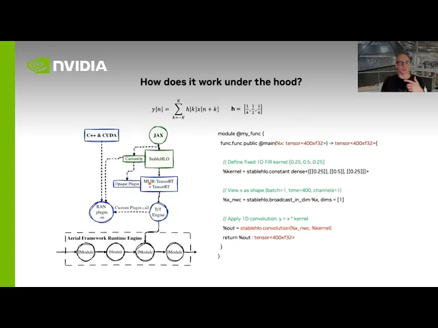
7:31 So how does it work under the hood?

7:33 So we start with our algorithm at the top here,

7:36 our finite impulse response filter.

7:38 We write it in JAX and then in JAX

7:41 we export the function to something called StableHLO

7:45 and StableHLO is a text representation of this function

7:50 that provides an intermediate representation for the compilers below.

7:54 Here you can see that X is an input tensor.

7:58 This is our X and for this example I

8:02 pass a length 400 of type float32 into the function.

8:05 It gets traced out through the function body.

8:09 And here you can see the kernel, the H,

8:13 becomes a StableHLO constant that more or less gets baked into the program.

8:19 And at the very bottom we have the operation defining the convolution.

8:24 And after the convolution,

8:25 the output tensor Y is returned of the same size and data type as the input.

8:33 So this text function StableHLO gets passed to our backend,

8:38 the ML TensorRT compiler,

8:39 which then compiles it down to a TensorRT engine that gets

8:45 injected into the Aerial Framework runtime that Michael was showing.

8:49 Now in addition to having this path for native Python code,

8:53 we have a path for high performance handwritten CUDA code as well.

8:57 So for example, if you have FFT or Cholesky or a solve operation that you

9:04 have a high performance implementation—could be LDPC

9:08 as well—we build it into a shared

9:11 library and then we expose it to JAX and StableHLO via the custom operation

9:15 and this gets passed down to the compiler

9:18 and this mechanism basically tells the compiler,

9:21 hey don't worry about it when you get to this function,

9:25 call out to this shared library and use that.

9:27 And this call is quite efficient, it takes a few microseconds to do.

9:33 So just to recap Michael's talk quickly, the runtime,

9:37 the product runtime, has this concept of pipelines and modules.

9:43 The modules are where we inject

9:46 our handwritten CUDA or our compiled TensorRT components.

9:51 The modules are the building blocks of the pipeline

9:56 and the pipeline coordinates the routing of information between these modules.

10:01 Now from the Python developer’s perspective, and to be honest my perspective,

10:07 what happens here is that I can put anything

10:10 I want from Python into a module via this TensorRT.

10:15 The only rules I need to follow are that the input data

10:19 types and the output data types match exactly what the C++ pipeline expects.

10:24 Of course.

10:25 So if you have a tensor of shape 400 and float32,

10:29 then you should accept 400 and float32 here.

10:32 And then of course the function that I write

10:34 in Python must compile successfully to a TensorRT engine.

10:37 But apart from that I can put anything I want into this pipeline

10:42 and then it gets executed on the GPU without any host CPU involvement.

10:47 So Michael showed this whole stack that comes

10:50 with the first release of Aerial Framework.

10:53 So we have the RU emulator, the NIC,

10:55 the fronthaul, and then the PUSCH receiver pipeline.

10:58 And this is the part I'm going to focus on in my talk.

11:01 So here there are two parts.

11:03 There's a PUSCH inner receiver and the PUSCH outer receiver.

11:08 The PUSCH inner receiver is shown in green

11:11 and the PUSCH outer receiver is shown in blue.

11:14 Now we have done this PUSCH outer receiver as a CUDA C++ set

11:19 of three modules and the reason for doing that, well there are two reasons.

11:24 First, we had a very high performance existing

11:27 implementation of the LDPC decoder already from Aerial cuPHY

11:31 and we wanted to test the workflow of mixing

11:36 development in CUDA with development exploratory research from Python.

11:41 So this is why we chose these two.

11:44 The Python side takes the inner receiver.

11:47 So we have the channel H,

11:49 the noisy received symbols, complex valued, coming in here.

11:53 We do DMRS extraction, channel estimation, interpolation,

11:57 interference plus noise covariance matrix estimation,

12:00 a standard MMSE-IC equalizer and soft mapper.

12:04 All of this gets compiled through the TensorRT compiler to a TensorRT

12:09 engine that becomes the first module in the Aerial Framework pipeline.

12:13 And on my machine, this gets about 90 microseconds plus a bit.

12:18 And Michael was showing around 200 microseconds.

12:21 So that's where we are there.

12:23 And for reference, this is for 100 megahertz bandwidth,

12:27 four receive antennas, one UE and one layer.

12:30 We do expect that this will scale very well with the number

12:34 of UEs given how the batching works for each of these operators.

12:39 So first up I did draw this in blue here

12:42 and the reason for that is because we actually use a custom plugin.

12:46 But before getting to that custom plugin

12:48 I'll just quickly refer to this figure here.

12:51 This is the DMRS configuration that we use for the test.

12:55 It's a standard one where the DMRS is on symbol two.

12:59 The DMRS sequence is on every second subcarrier.

13:02 The blue is the data that's transmitted from the user.

13:06 The gray is muted pilots that are not used.

13:09 So to create the DMRS sequence, we need to generate some random numbers.

13:14 And the way of doing that is to do this via two Gold sequences.

13:19 And this Gold sequence is generated

13:22 by having two linear feedback shift registers, this one here and this one here.

13:27 These are very sequential algorithms.

13:29 And when our first effort in prototyping this in JAX,

13:34 it worked and it compiled through.

13:36 However, the latency wasn't where we were at.

13:38 So we decided to write this as a custom CUDA plugin

13:43 where these feedback shift registers

13:45 were implemented essentially as lookup tables.

13:47 But this is a good way to highlight the workflow

13:50 where you start in JAX and then you can later,

13:55 when things harden, you can move to CUDA hardened kernels.

14:01 The next block in the PUSCH pipeline is channel estimation.

14:04 And there are many many ways to do channel estimation.

14:07 And what we've chosen here is a simple reference estimator

14:11 that is easy to calibrate and benchmark with our partners.

14:14 And the core idea is that you get the noisy DMRS in on this side.

14:19 You perform a least-squares channel estimate

14:22 to essentially extract or remove the DMRS symbols.

14:25 Then we have the raw and noisy channel in the frequency domain.

14:31 We do this IFFT to go to the time domain or delay domain.

14:37 We compute a power delay profile of the channel.

14:40 And then what happens is you get something like this black curve here.

14:44 So this represents the taps or the delays of the channel.

14:48 And then to perform filtering we perform a simple

14:52 threshold filter here where anything above the threshold we consider

14:57 to be the real channel and anything below we

15:01 consider to be noise and we set it to zero.

15:04 This threshold is simply based on the estimated noise power plus standard

15:07 deviation and then we've tuned some

15:09 hyperparameters to make it work reasonably okay.

15:12 After the thresholding we have the FFT back to the frequency domain.

15:17 To complete the inner receiver there are three more blocks.

15:20 There's the estimate of the interference

15:22 plus noise covariance matrix and this is done in the usual way by reconstructing

15:28 the desired signal from the received DMRS.

15:32 We compute the residuals.

15:34 So this is the error from the received DMRS minus the desired.

15:39 So it's the error from your estimate to what you received

15:43 and the covariance is computed in the normal way using an outer product.

15:49 We have this little optimization in there where

15:52 we apply this RBLW shrinkage method which essentially

15:55 uses a convex combination of two covariance matrices

16:00 to improve the accuracy of the covariance estimate.

16:04 And finally we have the standard MMSE-IC equalizer.

16:07 And for this we use a Cholesky

16:10 factor inverse method to compute this equation here.

16:14 Okay.

16:14 As Michael showed, this is what you'll get in the Nsight

16:19 Systems profiling tool when you run the full pipeline.

16:22 And you can see here for my machine we have about 10 microseconds for the DMRS.

16:27 And this includes the frequency orthogonal cover codes.

16:29 It also includes a casting of the channel,

16:32 a very large casting from float16 to float32.

16:36 And this is necessary because for the first release,

16:40 our FFTs for the channel estimator work with float32,

16:44 but the pipeline itself works with float16.

16:47 So there are some performance gains here immediately to have,

16:51 where we get some new kernels.

16:53 After the channel estimation we have the covariance estimation,

16:57 shrinkage and some transposes to prepare for the MMSE-IC equalizer.

17:02 And as Michael discussed when we zoomed into these things we

17:04 see that there are quite a few scatter-gather operations which suggests

17:07 that the way we did the data layout for the MMSE-IC can

17:11 be improved and there are some performance gains to be had here.

17:16 But nonetheless, for the first go implementing PUSCH from Python we,

17:22 in stream mode, have 185 or 186 microseconds latency.

17:28 Okay, so we have the PUSCH receiver in Python.

17:31 And for me, this is wonderful because it

17:33 means you can really start having fun and experimenting.

17:37 So if we take the channel estimator block here and then you go

17:42 after the DMRS extraction and you just look at the channel estimation part.

17:46 So I explained before first up that we have this weighted threshold,

17:51 this simple weighted threshold filter,

17:52 but immediately you can say well let's start trying other ideas.

17:56 So you just now plug in a different Python function to do this.

17:59 So in the first release we have one based on some

18:02 physics principles of free energy that we came up with.

18:05 I'm going to show you next the AI enhanced filter and in the notebook when you

18:10 run through there you'll see there'll be a cell

18:13 where you can define your own channel filter.

18:15 We gave a working example to get you started,

18:17 but in there you can just cut and paste and put your own ideas in and have

18:21 your filter compiled down with the rest of the chain

18:25 fused together and then profiled with everything else.

18:29 So the workflow in the notebook is

18:31 that you write your channel estimators in JAX,

18:33 export it to StableHLO and then you use this ML TensorRT

18:38 compiler to generate the engine that gets injected into the runtime pipeline.

18:43 And then we evaluate the performance of the channel

18:47 estimators using the 3GPP CDL-C model from SA.

18:51 And in the notebook, similar to what Michael showed,

18:55 you will get to profile what your channel

19:00 estimator does in a real product runtime type environment.

19:06 Okay.

19:06 So at the start of the talk, I talked about this idea of fusing

19:09 at a very deep level AI and classical algorithms.

19:12 So this is one idea or this is one example of that.

19:17 So here we have the same chain for channel estimation as I showed before.

19:22 We have the least-squares channel estimate.

19:24 We do an IFFT to go to the delay

19:27 domain and then we compute the power delay profile.

19:30 And before we would take this power delay profile here and we just threshold it

19:35 based on some heuristics to compute the FFT

19:38 and then FFT back to the frequency domain.

19:40 But instead of doing this thresholding based on heuristics,

19:43 what we can do is well let's use a more sophisticated filter.

19:48 So here we picked at random a Tukey

19:51 filter that is defined by these equations here.

19:54 And this filter has two parameters that define it, alpha and tau.

19:59 You can see alpha and tau define the shape

20:02 and how this filter is applied, where it's applied.

20:05 So instead of us hard coding, like you would in a classical system,

20:10 alpha and tau, we defined a neural network,

20:13 a transformer, to basically predict good values of alpha and tau

20:17 so that when you apply the filter it works well.

20:22 So when you train this, now that the whole thing

20:24 is written in JAX it means that we can compute

20:27 the mean squared error loss—actually it's a normalized mean squared

20:30 error that we use—of the true channel from Sionna versus

20:34 the estimate we get from our pipeline and we can

20:37 pass gradients all the way back through this pipeline to basically

20:41 optimize the transformer in such a way that it picks

20:45 good alpha and tau values to minimize this mean squared error.

20:50 And when you run the notebook and you train the AI model,

20:55 unfortunately we couldn't ship the pre-trained AI model,

20:57 so you'll have to train that one yourself.

21:00 You'll get a curve like this in the notebook.

21:03 On the x-axis, you have the SNR in dB ranging from minus 20

21:08 to 10 and on the y-axis you have the normalized mean squared error in dB.

21:13 So what we want is to get low values of the mean squared error.

21:18 So the lower the better.

21:20 And we can use that more or less as a rough proxy

21:24 to the single user uplink throughput you would experience on your mobile phone.

21:28 So lower here—so the red curve which is the AI

21:31 model performs a few dB better than the green curve,

21:35 which is this free energy idea, and that performs better than the Tukey filter.

21:40 I forgot to say that each one of these dots

21:43 is one particular channel realization for one particular filter.

21:47 So this is great.

21:50 The AI model beat the other ones, right?

21:53 But now that you have this ability to profile

21:57 the actual whole pipeline running on the product runtime,

22:01 you can look beyond this performance in MSE.

22:04 You can look at how long does it take to execute this model.

22:10 So we can see that the AI model takes 250 microseconds.

22:14 If we go down to the free energy model, it takes 169 microseconds.

22:18 This is not just for the channel filter.

22:21 Remember this is for DMRS generation and extraction,

22:25 the channel filtering and the covariance estimation as well.

22:29 But the point here is that now we can, as a researcher,

22:34 look at the model and we can look at how

22:37 the GPU is using that or how it's being executed

22:39 on the GPU and we can tailor the model fused

22:44 with the classical algorithms to get the most out of the GPU here.

22:52 Okay.

22:52 Yes.

22:52 So these are the settings.

22:54 You can look through the notebooks to see exactly what was run here.

22:58 So let's go deep into how we do this.

23:02 So at the backend we use this ML TensorRT compiler and this is

23:07 another open source project from NVIDIA that's been recently open sourced.

23:12 This compiler is for inference acceleration only.

23:15 It is not for training.

23:17 So it's just to accelerate during inference, during runtime.

23:21 The ML TensorRT compiler is for StableHLO programs.

23:26 So anything that can be expressed in StableHLO it can compile.

23:29 So we have a JAX frontend but you could

23:32 also use a Torch frontend with the Torch-MLIR pass.

23:36 We can also use TensorFlow as well.

23:40 Modularity means it integrates with existing ML compiler stacks.

23:44 One important thing is it has a TensorRT dialect.

23:49 So if we go to the compiler here,

23:51 this is the frontend of the compiler and at the backend it has several backends.

23:56 One is the TensorRT compiler and the other

23:59 is the Tiled IR and CodeGen compilers.

24:01 The TensorRT compiler is our main path.

24:04 So we traverse this link here.

24:07 And what the ML TensorRT compiler does is it provides a transpiler,

24:12 a conversion from our StableHLO representation of the function

24:16 to something that the TensorRT compiler understands

24:19 and then the TensorRT compiler is responsible for generating

24:23 the engine that gets injected into the runtime.

24:27 Okay.

24:27 So when you start playing with this there are some important things to note.

24:31 So if an operation or a data type is not supported by this TensorRT

24:36 compiler then what happens is you fall back to Tiled IR and CodeGen.

24:41 Now this is LLVM CodeGen, so this is not fully open sourced yet,

24:48 but the compiler will produce artifacts that you can use.

24:53 They'll produce PTX modules.

24:55 We don't at the moment have the ability—we have

24:57 not yet supported them in the Aerial Framework runtime.

25:00 That'll come in 2026.

25:02 So when you write your function, you should aim to use data types and operations

25:08 that are supported by the TensorRT compiler backend.

25:10 And you can look at the TensorRT website to see what is available there.

25:15 As it stands now, about 80% coverage of JAX ops is what we have.

25:21 But importantly it does not support many linear algebra operations,

25:25 namely solve, Cholesky, inverses, and FFT.

25:28 But this is no problem.

25:30 So what we have done is we've implemented

25:34 CUDA optimized kernels for these functions that we need

25:39 here and these get compiled into a shared

25:42 library that is made available or exposed to JAX

25:46 as a custom operation as I mentioned before

25:49 and this gets passed down to the compiler as an opaque

25:53 plugin and the compiler then can use this opaque

25:56 plugin as a reference when the TensorRT engine runs.

26:02 Complex data types—because TensorRT does not support complex data types,

26:06 they have to go via CodeGen.

26:07 So you'll get PTX for those and they won't

26:09 be able to immediately go into the Aerial Framework runtime.

26:12 But of course you could use them in your own C++ runtime if you wanted to.

26:17 If you want to use this compiler in your own standalone C++ project,

26:22 how we use it is via the EmitC runtime.

26:24 And this is what generates the TensorRT engine plus the PTX modules

26:28 and the C++ source to help you run the TensorRT engine and the PTX modules.

26:36 However, for the Aerial Framework we chose

26:39 to use our own integrations for the TensorRT engine.

26:44 So just to summarize what we've done in the development environment side.

26:50 First, this is available to anyone with a recent GPU.

26:55 It allows you to take JAX code or PyTorch code—we focused on JAX for the first

27:02 release—to compile that down to GPU executable code

27:06 that gets executed in GPU pipelines without host involvement.

27:10 Because we're working with Python and we can fuse in our own custom operators,

27:17 kernels like the DMRS generation for example or LDPC,

27:21 we can fuse at a very deep level

27:25 AI and signal processing and this fusion happens not

27:28 only at the algorithm level but as we

27:30 compile it down to an engine that gets executed,

27:33 it gets lowered to a single engine that gets executed in the pipeline.

27:38 And we think this is really fun to use

27:42 or to compile and deploy ideas in product trials,

27:46 test beds, or if you want just your simulators to run faster.

27:52 So what we have is our JAX implementation

27:55 of the inner receiver with a few plugins.

27:59 It gets compiled through TensorRT.

28:01 How I did it was we profiled a lot using nsys.

28:05 We iterated and optimized as much as we could with the time we had and then we

28:12 injected it directly into the Aerial Framework runtime

28:17 engine here and ran the thing end to end.

28:23 So what's next?

28:24 Well, we'll continue working on this problem of lowering

28:29 Python and we'll experiment and share technologies around this.

28:33 The DSLs we're focusing on are JAX, PyTorch,

28:36 and CuTe Tile that was recently open sourced by NVIDIA.

28:41 And we're focusing of course on Aerial Framework’s runtime.

28:44 We'll continue to work with the ML TensorRT compiler alongside

28:49 the new ways of working with CuTe Tile and Tiled IR.

28:53 I'm very interested in the ability

28:55 to manually write and fuse signal processing kernels.

28:59 So if you have two heavy matrix operations in Python

29:04 and you want to write a kernel directly that's fused,

29:08 where you specify the GPU tile size and all the rest,

29:13 making that available in Python so you can quickly prototype and compile

29:16 it down to something that can be injected into the Aerial Framework runtime.

29:21 We'll be evaluating integration with Sionna via TensorFlow.

29:25 We'll continue to build up our performant kernels such as DMRS,

29:29 FFT, Cholesky, and so on.

29:31 And over the coming months,

29:33 we're going to complete the missing PHY pipelines to add

29:37 the standard-essential features needed to go over the air sometime in 2026.

29:41 And of course, we're going to optimize, optimize,

29:45 and optimize to see how fast this AI-native Python based framework can take us.

29:52 This is available on GitHub from today.

29:55 We'll share our progress regularly and it

30:00 will be wonderful to get feedback from you.

30:07 That's it.

30:09 Thank you.

30:11 Got lots of questions.

30:13 So we're going to give it a go to see how many

30:16 of those questions we can get through in the remaining time that we have.

30:22 So I think, let me attempt grouping the questions

30:26 so that we have some consistency in terms of answering.

30:30 So you can expect there are questions around the software,

30:33 there are questions around the hardware,

30:36 there are also questions about relationship with other NVIDIA tool sets.

30:41 So let me take the first one here and wrap it

30:46 around a few of the other questions that I'm seeing here.

30:49 What's the hardware required for a developer environment in this case?

30:54 So for the development side, any modern recent GPU.

30:59 I think the official thing is we've said compute capability 8 or above.

31:06 So I've tested this on the GH100, GH200, RTX 6000, and RTX 5090.

31:15 We haven't tested on Spark that much yet.

31:22 Okay.

31:22 Okay, it's good.

31:24 Thank you.

31:25 And let me read it directly from how it's

31:29 come in so that hopefully I don't begin to paraphrase.

31:34 Two questions around CUDA and C++ code.

31:38 I'll take the first one.

31:41 Is it possible to use this signal processing toolkit to, is it, sorry,

31:49 is it possible to use Aerial to generate C++ code that is compatible with cuBB?

31:58 Yeah, I mean there's no generation of the C++.

32:02 But what we did do, say for the DMRS example,

32:07 is to take the optimized DMRS CUDA kernel

32:11 from cuPHY and you can write any kernel you like.

32:17 So for example we wrote one for FFT and another for Cholesky inverse that is

32:25 written in CUDA C++ and you would compile

32:28 that down to that shared library I showed.

32:30 So at the moment there is no code generation for C++ CUDA,

32:34 but of course if you have your own toolchain, if you have your own framework,

32:41 generative AI framework or whatever to generate the CUDA kernels,

32:45 then of course you can have the kernels generated that way

32:50 and use them as plugins like we did for DMRS and FFT.

32:55 Okay, fantastic.

32:56 I've got another question here that's going into detail.

33:01 So I think what they're trying to understand here is a clarification of why,

33:07 you know, with the development language of choice of CUDA C++.

33:12 So the person: can you please explain once

33:15 again for the development language choice of CUDA C++

33:20 for PUSCH outer receiver versus a TensorRT engine for PUSCH

33:24 inner receiver and the reasons for making these choices.

33:30 Ah okay.

33:32 Yes.

33:33 So this was this choice.

33:36 So we chose Python for this inner receiver.

33:40 I didn't explain this so this is good.

33:43 Because there's a lot of research

33:45 and innovation going around AI-based channel estimators.

33:48 And in the first talk today from the Sionna team

33:53 they talked about their neural receiver that combines channel estimator,

33:59 interference covariance estimation and equalizer

34:01 all into one big neural network.

34:03 So there's a lot of research and exploratory stuff going around here.

34:07 So this is very good to have in Python to have flexibility.

34:11 On the backend here in the outer receiver,

34:15 the LDPC decoder is quite fixed, right?

34:19 In 5G and in 6G I guess it's going to be quite

34:21 similar and we had a very very high performant LDPC decoder already.

34:25 So to help us go over the air we took that implementation.

34:30 That was one part of the reason and the other was we wanted to test

34:34 this workflow of having a mix of CUDA

34:36 C++ and this Python in the same pipeline, right?

34:39 We had to build the framework around to make this work.

34:43 Okay.

34:44 Okay, thank you.

34:45 Another question here is asking for you to flesh out a bit more.

34:51 What are the benefits of using GPU compute for this?

34:57 The benefits of using GPU—yeah,

35:00 I mean for me it is this flexibility in the platform

35:07 and the software development tools that we have on top.

35:12 If you were to, I mean what we did here

35:15 is we basically took a Python implementation of the PUSCH receiver,

35:19 which is one of the most extreme uses in the RAN,

35:23 and we made it run almost at product level latencies.

35:27 And this was only possible because we have

35:31 this huge ecosystem of CUDA software to build on.

35:34 We didn't build this ML TensorRT compiler;

35:37 we worked a lot with their team but we didn't build it,

35:41 like these are some great guys behind

35:43 that building that and underneath that there

35:45 is the TensorRT compiler and then underneath

35:47 that you have all sorts of great developments.

35:51 So this is one advantage that is very hard

35:57 to overcome if you want to work on GPU platforms.

36:03 This is wonderful.

36:05 Okay.

36:05 Yeah.

36:06 And looking at the DMRS parameters that you didn't show here.

36:14 So how are those handled?

36:18 Right.

36:19 So here we have just the channel coming in here.

36:23 But of course there are many parameters needed

36:27 to set up this pipeline and these parameters can

36:30 be passed in as dynamic inputs or they

36:33 can be compiled as static inputs in the pipeline.

36:36 And in the notebook you'll see how to do that.

36:39 How to fix some parameters as dynamic that change from slot to slot

36:44 or have others fixed to static that are held constant in the engine itself.

36:52 Okay.

36:52 Okay.

36:53 I'm looking at questions here regarding data types.

36:57 So someone is asking, you know,

37:00 can we use complex data types or what type of data types are supported?

37:07 I mean the architecture of this pipeline, is that what's meant here?

37:12 I think so.

37:13 Correct me if that's not right.

37:16 So I think it's any directed acyclic graph that we can have here.

37:23 So here we keep just a, I guess,

37:25 a linear pipeline from one module to the next but the framework supports,

37:31 you can have more complicated structures here for sure.

37:38 Okay.

37:38 Okay.

37:39 And what part of this transmission

37:42 receiver pipeline was accelerated most drastically?

37:47 Um I mean we went from Python which takes,

37:55 I mean I think, I don't remember the numbers.

37:58 This maybe ran in half a second if you run it

38:01 in Python or something and we took it down to 190 microseconds.

38:05 So this is a big acceleration here.

38:08 This side has been optimized and optimized and optimized

38:12 by the Aerial team for the last number of years.

38:17 So this is already very highly performant but of course it's super accelerated.

38:24 I guess that explains some of the questions that have just been coming in now.

38:29 One of the questions is, you know, you're showing us the PUSCH receiver.

38:34 Any work on the PDSCH receiver as well?

38:38 Yes.

38:38 We'll have that one soon.

38:40 Yes, we need that one to go over the air.

38:44 So that's in the pipeline.

38:46 We just weren't ready.

38:47 We weren't ready for the first release with PDSCH.

38:50 I see.

38:50 Another one related to what you have on screen there about the LDPC decoder.

38:57 Is it open source?

38:59 How efficient is it?

39:04 I don't know the exact,

39:06 it's part of the Aerial SDK and I will leave it to someone

39:09 else to answer the exact open-source nature of the details of the LDPC decoder.

39:16 But it is very efficient.

39:19 Yes.

39:19 Okay.

39:20 Let me get more of the questions as well.

39:24 So somebody's asking us here,

39:27 can I use compiled Python with my own C++ simulator?

39:33 Yeah, absolutely.

39:34 And that's how I started.

39:37 So when we started, before we had this pipeline built,

39:41 we started prototyping this in Python and compiling it down.

39:46 And when you compile it with this compiler using the EmitC backend,

39:50 it will generate C++ host code for you

39:53 to show you how to stitch together the different artifacts,

39:56 the TensorRT engines, the PTX modules and so on, how to stitch them together.

40:01 And I had my own C++ pipeline testing this.

40:04 So of course if you have a C++ simulator with a GPU and you

40:10 want to offload some things to that, yes of course you can use this compiler.

40:17 You can use our helpers,

40:20 our wrappers for that compiler as standalone for your C++.

40:24 Yes.

40:25 Okay.

40:25 Let's talk a bit about JAX because I'm seeing questions here.

40:29 So why did you use JAX?

40:31 Well, answer that before I get to the next

40:34 question because the person had two questions,

40:37 well two different people asking about JAX.

40:39 So why did you use JAX?

40:40 Then I'll come to the next question on JAX.

40:43 First, for people who know me they know I like JAX very much.

40:48 So maybe there's a bias.

40:51 But the real reason was JAX has this ability—I mean we export

40:57 to StableHLO and here with the ML TensorRT compiler we get this nice flow

41:03 and this compiler handled complex numbers out of the box and it had a lot

41:10 broader support than what we could get

41:13 with PyTorch directly with the TensorRT backend.

41:16 So that was the original motivation for using JAX.

41:22 Then the second benefit came from having these custom ops registered with JAX.

41:27 So this is a really wonderful way that JAX was built that you can register

41:33 my DMRS plugin as a native operation in JAX and the Python user just writes,

41:38 I want DMRS here, but under the hood the compiler knows

41:42 how to handle that and go to the custom CUDA kernel.

41:46 That being said, we also like PyTorch very much and we are working

41:51 on a way of having a PUSCH receiver or a way of working with PyTorch directly.

41:57 And there are a number of different options

42:00 and we have some examples in the codebase already.

42:03 You can use the TensorRT API directly

42:06 to build up the layers of the TensorRT engine

42:11 directly with PyTorch or you can use PyTorch-MLIR

42:16 to go via StableHLO like we did with JAX.

42:20 Okay.

42:21 So is it only the, so what parts of the RAN pipeline can be JAX compiled?

42:30 Is it only the AI block or also some classical DSP kernels?

42:37 No, I mean the whole, all of this is JAX.

42:40 So the DMRS extraction, the channel estimator, the classical methods,

42:44 the AI method, the mixed method, this is all JAX.

42:49 This interference plus noise covariance matrix estimation, this is JAX.

42:53 The MMSE-IC equalizer is all JAX except

42:55 the custom call to the Cholesky factorization.

42:58 The soft mapper is all JAX.

43:01 So all these are classical algorithms and they're all written in JAX.

43:05 Okay, I'm trying to pull up all the questions around

43:09 PyTorch because I've seen a few of them come through.

43:16 Okay.

43:17 So can we use PyTorch?

43:20 Yes absolutely.

43:21 So when you use, the way to use PyTorch, there are two ways.

43:26 If you want to use it with the ML TensorRT compiler

43:30 then you use something called Torch-MLIR and you export your Torch

43:35 model to StableHLO and then you hand it over to this compiler

43:38 in the same way as what we do for JAX.

43:43 And I think we have an example in the codebase.

43:46 I should double check that.

43:48 But at least we did in testing where we had

43:52 a PyTorch function exported by MLIR in StableHLO and this compiler.

43:58 That's the first way.

44:02 The second way is to use the TensorRT interfaces directly from PyTorch.

44:12 That's also possible and we have an example in the code base how to do that.

44:18 Okay, let's talk about latency here.

44:22 How close is the receiver latency with respect

44:26 to handwritten CUDA from our cuPHY library?

44:31 So I mean we were somewhere around—this was stream mode—180 or so.

44:39 We think there's some improvements, we're around 150.

44:43 The handwritten optimized CUDA implementation in cuPHY on this machine

44:49 for this workload was around 50 or 60 microseconds.

44:54 So we're getting closer and closer.

44:57 But of course with a lot more flexibility.

45:02 Okay.

45:03 Okay.

45:03 I'm trying to see if I can pull up

45:06 just another latency question that I want to find.

45:09 Okay, I don't think I can find it, but it's one of those that we will

45:15 provide an answer after the event and come back.

45:19 Okay, another question on PUSCH receiver.

45:22 So, it says, can you introduce more AI algorithms used

45:26 to improve the performance of the PUSCH receiver except for channel estimation?

45:30 Yeah, of course.

45:32 I'm looking forward to working with the SA team,

45:35 for example, to do a full neural receiver.

45:37 So where we combine all of these together and build up the neural network,

45:43 whether it be convolution based or transformer based,

45:47 and then see how fast we can make it run on the GPU.

45:53 So yes, because this is written all

45:56 in JAX it means it's all differentiable which

45:59 means that anything that you can differentiate

46:01 is fair game for doing machine learning optimizations.

46:05 So if you can figure out a way to optimize the soft mapper,

46:10 yeah go for it and run gradient descent because it's differentiable.

46:14 Yeah.

46:14 Okay.

46:15 And could this model run efficiently on DUs with GPU/DPU acceleration?

46:24 Yes, that's our hope,

46:26 that you will be able to deploy some code to a test bed DU or a product DU,

46:34 try it out and see if it works.

46:37 And then maybe you can hand write some

46:40 things to harden it to get the ultimate performance.

46:43 Or maybe you want a machine learning model

46:46 in there that you want to be updated regularly,

46:48 in which case that would probably stay as a TensorRT engine and stay in Python.

46:54 Okay.

46:54 And maybe we close off with one final question.

46:59 Are you accepting contributions on GitHub?

47:02 I guess lots of people want to get their hands busy with this.

47:08 What's the plan?

47:10 We're not quite ready to accept contributions, but we'd love to get feedback.

47:19 And I guess we'll work towards that.

47:24 Okay.

47:24 Okay.

47:25 Let me see if there's any other one that I could—oh, yeah, another one.

47:33 Maybe hopefully we close out on that.

47:36 Can we use this with Sionna?

47:39 We're working towards that now.

47:41 Sionna is based on TensorFlow

47:44 and the compiler can compile TensorFlow to StableHLO.

47:48 Though we have to look at the specific operations.

47:52 Sionna is a very rich and wonderful library.

47:55 We have to look at the particular operations and data types they use to see

48:00 how practical it is to take a big block of Sionna and just drop it in.

48:05 We're working through those details.

48:08 Okay.

48:08 Okay.

48:09 I think we begin to wrap it up there.

48:13 So thank you very much, Roy, for walking us through all of that.