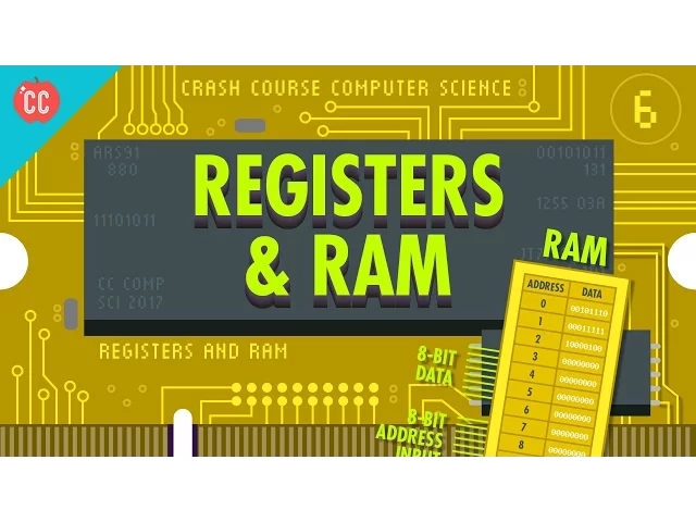
Registers and RAM: Crash Course Computer Science #6

0:03 Hi, I’m Carrie Anne and welcome to Crash Course Computer Science.

0:05 So last episode, using just logic gates, we built a simple ALU,

0:09 which performs arithmetic and logic operations, hence the ‘A’ and the ‘L’.

0:13 But of course, there’s not much point in calculating a result only

0:16 to throw it away- it would be useful to store that value somehow,

0:20 and maybe even run several operations in a row.

0:22 That's where computer memory comes in!

0:24 If you've ever been in the middle of a long RPG campaign on your console,

0:28 or slogging through a difficult level on Minesweeper on your desktop,

0:31 and your dog came by, tripped and pulled the power cord out of the wall,

0:34 you know the agony of losing all your progress.

0:36 Condolences.

0:38 But the reason for your loss is that your console,

0:40 your laptop and your computers make use of Random Access Memory,

0:43 or RAM, which stores things like game state- as long as the power stays on.

0:47 Another type of memory, called persistent memory, can survive without power,

0:51 and it’s used for different things;

0:52 We'll talk about the persistence of memory in a later episode.

0:55 Today, we’re going to start small- literally

0:57 by building a circuit that can store one..

1:00 single..

1:00 bit of information.

1:01 After that, we’ll scale up, and build our very own memory module,

1:04 and we’ll combine it with our ALU next time,

1:07 when we finally build our very own CPU!

1:10 INTRO All of the logic circuits we've discussed so far go in one

1:22 direction- always flowing forward- like

1:24 our 8-bit ripple adder from last episode.

1:26 But we can also create circuits that loop back on themselves.

1:29 Let’s try taking an ordinary OR gate,

1:31 and feed the output back into one of its inputs and see what happens.

1:35 First, let’s set both inputs to 0.

1:37 So 0 OR 0 is 0, and so this circuit always outputs 0.

1:41 If we were to flip input A to 1.

1:44 1 OR 0 is 1, so now the output of the OR gate is 1.

1:48 A fraction of a second later, that loops back around into input B,

1:51 so the OR gate sees that both of its inputs are now 1.

1:54 1 OR 1 is still 1, so there is no change in output.

1:58 If we flip input A back to 0, the OR gate still outputs 1.

2:01 So now we've got a circuit that records a “1” for us.

2:04 Except, we've got a teensy tiny problem- this change is permanent!

2:07 No matter how hard we try,

2:09 there’s no way to get this circuit to flip back from a 1 to a 0.

2:13 Now let’s look at this same circuit, but with an AND gate instead.

2:16 We'll start inputs A and B both at 1.

2:19 1 AND 1 outputs 1 forever.

2:21 But, if we then flip input A to 0,

2:23 because it’s an AND gate, the output will go to 0.

2:26 So this circuit records a 0, the opposite of our other circuit.

2:29 Like before, no matter what input we apply to input A afterwards,

2:33 the circuit will always output 0.

2:34 Now we’ve got circuits that can record both 0s and 1s.

2:38 The key to making this a useful piece of memory is

2:40 to combine our two circuits into what is called the AND-OR Latch.

2:44 It has two inputs, a "set" input, which sets the output to a 1,

2:47 and a "reset" input, which resets the output to a 0.

2:50 If set and reset are both 0,

2:52 the circuit just outputs whatever was last put in it.

2:54 In other words, it remembers a single bit of information!

2:58 Memory!

2:59 This is called a “latch” because it “latches

3:01 onto” a particular value and stays that way.

3:03 The action of putting data into memory is called writing,

3:06 whereas getting the data out is called reading.

3:09 Ok, so we’ve got a way to store a single bit of information!

3:12 Great!

3:13 Unfortunately, having two different wires for input–

3:15 set and reset– is a bit confusing.

3:18 To make this a little easier to use, we really want a single wire to input data,

3:22 that we can set to either 0 or 1 to store the value.

3:24 Additionally, we are going to need a wire that enables the memory to be

3:28 either available for writing or “locked” down

3:30 --which is called the write enable line.

3:32 By adding a few extra logic gates, we can build this circuit,

3:35 which is called a Gated Latch since the “gate” can be opened or closed.

3:39 Now this circuit is starting to get a little complicated.

3:41 We don’t want to have to deal with all the individual logic gates...

3:44 so as before, we’re going to bump up a level of abstraction,

3:46 and put our whole Gated Latch circuit in a box— a box that stores one bit.

3:50 Let’s test out our new component!

3:52 Let’s start everything at 0.

3:54 If we toggle the Data wire from 0 to 1 or 1 to 0,

3:58 nothing happens- the output stays at 0.

4:00 That’s because the write enable wire is off,

4:02 which prevents any change to the memory.

4:04 So we need to “open” the “gate” by turning the write enable wire to 1.

4:07 Now we can put a 1 on the data line to save the value 1 to our latch.

4:11 Notice how the output is now 1.

4:14 Success!

4:14 We can turn off the enable line and the output stays as 1.

4:18 Once again, we can toggle the value on the data line all we want,

4:21 but the output will stay the same.

4:22 The value is saved in memory.

4:24 Now let’s turn the enable line on again use our data line to set the latch to 0.

4:29 Done.

4:30 Enable line off, and the output is 0.

4:32 And it works!

4:33 Now, of course, computer memory that only stores one bit

4:36 of information isn’t very useful— definitely not enough to run Frogger.

4:39 Or anything, really.

4:41 But we’re not limited to using only one latch.

4:43 If we put 8 latches side-by-side,

4:45 we can store 8 bits of information like an 8-bit number.

4:48 A group of latches operating like this is called a register,

4:51 which holds a single number,

4:53 and the number of bits in a register is called its width.

4:56 Early computers had 8-bit registers, then 16, 32,

4:59 and today, many computers have registers that are 64-bits wide.

5:03 To write to our register, we first have to enable all of the latches.

5:06 We can do this with a single wire that connects

5:09 to all of their enable inputs, which we set to 1.

5:11 We then send our data in using the 8 data wires,

5:14 and then set enable back to 0, and the 8 bit value is now saved in memory.

5:19 Putting latches side-by-side works ok for a small-ish number of bits.

5:23 A 64-bit register would need 64 wires running to the data pins,

5:27 and 64 wires running to the outputs.

5:29 Luckily we only need 1 wire to enable all the latches,

5:34 but that’s still 129 wires.

5:36 For 256 bits, we end up with 513 wires!

5:40 The solution is a matrix!

5:42 In this matrix, we don’t arrange our latches in a row, we put them in a grid.

5:46 For 256 bits, we need a 16 by 16

5:49 grid of latches with 16 rows and columns of wires.

5:52 To activate any one latch,

5:54 we must turn on the corresponding row AND column wire.

5:56 Let’s zoom in and see how this works.

5:58 We only want the latch at the intersection

6:00 of the two active wires to be enabled,

6:02 but all of the other latches should stay disabled.

6:05 For this, we can use our trusty AND gate!

6:08 The AND gate will output a 1 only if the row and the column wires are both 1.

6:12 So we can use this signal to uniquely select a single latch.

6:15 This row/column setup connects all our latches with a single,

6:19 shared, write enable wire.

6:20 In order for a latch to become write enabled, the row wire,

6:23 the column wire, and the write enable wire must all be 1.

6:26 That should only ever be true for one single latch at any given time.

6:29 This means we can use a single, shared wire for data.

6:32 Because only one latch will ever be write enabled,

6:35 only one will ever save the data— the rest of the latches will

6:38 simply ignore values on the data wire because they are not write enabled.

6:41 We can use the same trick with a read enable wire to read the data later,

6:45 to get the data out of one specific latch.

6:48 This means in total, for 256 bits of memory, we only need 35 wires- 1 data wire,

6:54 1 write enable wire, 1 read enable wire,

6:57 and 16 rows and columns for the selection.

6:59 That’s significant wire savings!

7:01 But we need a way to uniquely specify each intersection.

7:05 We can think of this like a city,

7:06 where you might want to meet someone at 12th avenue

7:08 and 8th street— that's an address that defines an intersection.

7:11 The latch we just saved our one bit into has an address of row 12 and column 8.

7:15 Since there is a maximum of 16 rows, we store the row address in a 4 bit number.

7:20 12 is 1100 in binary.

7:23 We can do the same for the column address: 8 is 1000 in binary.

7:28 So the address for the particular latch we just used can be written as 11001000.

7:35 To convert from an address into something that selects the right row or column,

7:38 we need a special component called a multiplexer— which is the computer

7:41 component with a pretty cool name at least compared to the ALU.

7:45 Multiplexers come in all different sizes, but because we have 16 rows,

7:48 we need a 1 to 16 multiplexer.

7:51 It works like this.

7:52 You feed it a 4 bit number,

7:53 and it connects the input line to a corresponding output line.

7:56 So if we pass in 0000, it will select the very first column for us.

8:02 If we pass in 0001, the next column is selected, and so on.

8:06 We need one multiplexer to handle our rows

8:08 and another multiplexer to handle the columns.

8:10 Ok, it’s starting to get complicated again,

8:13 so let’s make our 256-bit memory its own component.

8:16 Once again a new level of abstraction!

8:24 It takes an 8-bit address for input- the 4

8:27 bits for the column and 4 for the row.

8:29 We also need write and read enable wires.

8:32 And finally, we need just one data wire,

8:34 which can be used to read or write data.

8:37 Unfortunately, even 256-bits of memory isn’t enough to run much of anything,

8:41 so we need to scale up even more!

8:43 We’re going to put them in a row.

8:45 Just like with the registers.

8:46 We’ll make a row of 8 of them,

8:48 so we can store an 8 bit number- also known as a byte.

8:51 To do this, we feed the exact same address into all

8:55 8 of our 256-bit memory components at the same time,

8:58 and each one saves one bit of the number.

9:01 That means the component we just made

9:04 can store 256 bytes at 256 different addresses.

9:07 Again, to keep things simple, we want to leave behind this inner complexity.

9:11 Instead of thinking of this as a series

9:13 of individual memory modules and circuits,

9:15 we’ll think of it as a uniform bank of addressable memory.

9:18 We have 256 addresses, and at each address, we can read or write an 8-bit value.

9:23 We’re going to use this memory component next episode when we build our CPU.

9:28 The way that modern computers scale to megabytes

9:30 and gigabytes of memory is by doing the same thing we’ve been doing here— keep

9:34 packaging up little bundles of memory into larger,

9:36 and larger, and larger arrangements.

9:37 As the number of memory locations grow, our addresses have to grow as well.

9:42 8 bits hold enough numbers to provide addresses

9:45 for 256 bytes of our memory, but that’s all.

9:48 To address a gigabyte– or a billion bytes of memory– we need 32-bit addresses.

9:53 An important property of this memory is that we can access any memory location,

9:57 at any time, and in a random order.

9:59 For this reason, it’s called Random-Access Memory or RAM.

10:03 When you hear people talking about how much

10:05 RAM a computer has- that's the computer’s memory.

10:07 RAM is like a human’s short term or working memory,

10:09 where you keep track of things going on right now- like

10:12 whether or not you had lunch or paid your phone bill.

10:14 Here’s an actual stick of RAM- with 8 memory modules soldered onto the board.

10:18 If we carefully opened up one of these modules and zoomed

10:20 in, The first thing you would see are 32 squares of memory.

10:23 Zoom into one of those squares,

10:25 and we can see each one is comprised of 4 smaller blocks.

10:28 If we zoom in again, we get down to the matrix of individual bits.

10:31 This is a matrix of 128 by 64 bits.

10:34 That’s 8192 bits in total.

10:37 Each of our 32 squares has 4 matrices,

10:40 so that’s 32 thousand, 7 hundred and 68 bits.

10:43 And there are 32 squares in total.

10:45 So all in all, that’s roughly 1 million bits of memory in each chip.

10:49 Our RAM stick has 8 of these chips, so in total,

10:52 this RAM can store 8 millions bits, otherwise known as 1 megabyte.

10:56 That’s not a lot of memory these days— this is a RAM module from the 1980’s.

11:00 Today you can buy RAM that has a gigabyte

11:03 or more of memory- that’s billions of bytes of memory.

11:06 So, today, we built a piece

11:08 of SRAM- Static Random-Access Memory– which uses latches.

11:11 There are other types of RAM, such as DRAM, Flash memory, and NVRAM.

11:15 These are very similar in function to SRAM,

11:17 but use different circuits to store the individual bits— for example,

11:20 using different logic gates, capacitors, charge traps, or memristors.

11:24 But fundamentally, all of these technologies store bits

11:27 of information in massively nested matrices of memory cells.

11:31 Like many things in computing, the fundamental operation is relatively simple..

11:34 it’s the layers and layers of abstraction that’s mind blowing— like

11:38 a russian doll that keeps getting smaller and smaller and smaller.

11:42 I’ll see you next week.

11:44 Credits