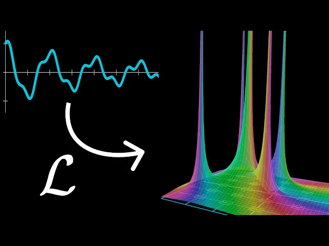
But what is a Laplace Transform?

0:00 [Submit subtitle corrections at criblate.com] What

0:01 you're looking at, a somewhat complicated

0:02 diagram that you and I are going to build up in this video,

0:05 is a visualization unpacking the meaning behind one

0:08 of the most powerful tools used to study differential equations.

0:12 It's known as the Laplace transform.

0:18 This is one of those tools where, as a student,

0:20 you can learn how to use it to solve equations,

0:23 and yet be left completely in the dark about what it's actually doing.

0:26 Think about learning how to drive a car

0:29 versus learning how an internal combustion engine works.

0:32 Both are worthy pursuits, one is not necessarily better than the other,

0:36 and in fact driving is probably more practical.

0:39 But there is something deeply satisfying about popping

0:42 open the hood and understanding the mechanism inside.

0:45 Similarly, our main goal with this video is to pop the hood

0:49 and show you some of the beautiful math that awaits us inside this object.

0:54 And strictly speaking, a lot of what I want to show is

0:56 not necessary if your only goal is to solve equations.

1:00 That said, for the differential equation students among you,

1:02 I think the content here should make the stuff

1:05 you have to memorize a lot more memorable, and after dissecting this machine,

1:08 studying it piece by piece,

1:10 you and I will take everything for a test drive and see

1:12 what it looks like to solve

1:13 a concrete and very interesting differential equation.

1:17 Now before I just plop down the definition on the screen,

1:20 let's talk about what problem the Laplace transform is trying to solve.

1:24 We set up a lot of this in the previous chapter,

1:27 and there are two primary ideas worth restating here.

1:30 Number one, you need to understand exponential functions,

1:33 and I'm always going to be writing these as e^(st) t represents time,

1:38 and then s is a number.

1:41 It determines what specific exponential we're talking about,

1:44 but very importantly for this topic,

1:45 we're going to give s the freedom to take on complex number values.

1:50 We covered this much more thoroughly in the previous chapter,

1:53 but the quick summary is that if s has an imaginary part,

1:56 the output of your function rotates in the complex plane as time ticks forward.

2:01 When the real part of s is negative,

2:03 the magnitude is decaying towards zero over time,

2:06 but if it happens to be positive,

2:08 that would mean the magnitude grows, namely growing exponentially.

2:12 If any of that feels shaky or if you want to understand why it's true,

2:15 do watch the previous chapter, but from this point forward,

2:18 I'm assuming everybody is comfortable with this notion.

2:22 Why do we care, though?

2:23 Why the hubbub about these functions?

2:25 Well, it's because of the second thing you need to know,

2:28 which is that a lot of functions, especially those arising in physics,

2:31 can be expressed as combinations of exponential pieces.

2:35 There's one very friendly example that's going to be helpful

2:38 to return to repeatedly throughout this lesson, the cosine of t.

2:41 This undulating function can be broken up

2:44 as a sum of two purely imaginary exponentials.

2:48 Basically, if you take e^(it), that gives you rotation counterclockwise,

2:52 and e^(-it) rotates the other way, so when you add these two together,

2:57 perhaps imagining adding two rotating vectors tip to tail,

3:00 the imaginary parts cancel each other out,

3:02 and what you're left with is something whose

3:05 output remains locked to the real number line, oscillating back and forth.

3:10 Now as it stands, this sum goes between negative two and positive two,

3:14 but a cosine only goes between negative one and one,

3:17 so finally you multiply everything by one half.

3:22 More complicated functions might break down into more exponential pieces.

3:26 For example, later in this lesson,

3:27 you and I are going to dig into something called the driven harmonic oscillator,

3:31 which is basically a mass on a spring that's influenced by some external force,

3:36 in our case, one that oscillates over time.

3:38 As a spoiler, the solution to the equation describing

3:41 that ends up looking like a sum of four exponential pieces.

3:46 Two of those pieces oscillate and decay in a way

3:48 that matches the natural resonant frequency of the spring,

3:51 and then the other two oscillate in a way that matches the external force.

3:56 So for cases like this and many others, what we would like is some sort of tool,

4:00 some sort of mathematical machine where you can pump in a function,

4:04 or even a differential equation describing that function,

4:07 and that machine will somehow reveal for us

4:10 what specific exponential pieces that function breaks down into.

4:14 That is, it exposes what these values s in the exponent all are,

4:17 as well as what the corresponding coefficients are.

4:20 Now you might be wondering why exponential pieces,

4:23 why not focus on something else.

4:25 The short answer is that for these functions, when you take a derivative,

4:29 it looks precisely the same as multiplying by some number, namely s.

4:34 What you'll see by the end is how this means that same machine that lets

4:38 us dissect functions into exponential pieces also

4:41 allows us to turn differential equations into algebra,

4:45 essentially because everywhere you see a derivative,

4:48 it turns into multiplication by s.

4:52 Now in a context like this one

4:54 where we are so focused on complex-valued exponentials,

4:57 engineers have a special name for this complex

4:59 plane that I'm depicting on the left,

5:02 representing all possible values for that term s in the exponent.

5:06 They call it, well, the s-plane.

5:09 A helpful mental image is to think of each individual

5:13 point on the s-plane as encoding the entire exponential function e^(st).

5:19 For this picture, the graphs I'm showing

5:21 only depict the real component of the output,

5:24 but keep in mind, each point is representing the full complex-valued function.

5:28 These graphs are enough for intuition though.

5:30 You'll notice how bigger imaginary parts correspond to faster oscillation,

5:35 and then as your eyes scan from left to right,

5:37 the real part reflects either decay or growth.

5:42 So with this as our goal,

5:43 the machine that you and I are going to build up today,

5:46 the one that exposes how a function breaks into exponential pieces,

5:49 is, as you have no doubt guessed, the Laplace transform.

5:53 Now this word transform is a little funny,

5:56 basically in the same way that a function is something

5:59 that takes in a number and spits out a new number,

6:02 we often use the word transform in math for a more meta

6:06 operation that takes in an entire function and spits out a new function.

6:11 In the case of the Laplace transform,

6:13 a typical convention is to name our new function with a capitalized

6:16 version of whatever you use to name that original function.

6:20 And in this setting, where our original function takes in time as an input,

6:25 the new transformed function has a new

6:28 different kind of input, a complex value, s.

6:31 I think it's helpful to quickly preview what this new function

6:34 actually does before we pull up the definition and start dissecting it.

6:38 Suppose your original function, f(t),

6:41 really can be broken down as a sum of several exponential pieces.

6:46 When you apply this Laplace transform,

6:48 giving you a new function of this new variable s,

6:51 if you were to plot this new function over the s plane,

6:54 in a way that I will explain in just a minute,

6:57 what you see are these sharp spikes above each value

7:00 of s that corresponds to one of those exponential pieces.

7:05 These spikes have a fancy name, they are called the poles of your function.

7:09 So even if you didn't know ahead of time how

7:12 your function could be broken down as a sum of exponentials,

7:15 if you understand this transformed version,

7:18 and specifically if you understand the poles,

7:21 that can reveal for you what those exponential pieces are.

7:25 At this point you're probably itching to see how this thing is actually defined,

7:29 and in its full glory this is what that definition looks like,

7:32 which we can think of as two separate steps.

7:35 First, you multiply your function by the expression e^(-st), and then second,

7:40 you integrate that result over time from t equals zero to infinity.

7:46 We'll talk all about that integral and its nuances in just a minute,

7:49 but for the moment focus on that inner expression.

7:52 This term s is the newly introduced parameter,

7:54 the one that is the input of our new transformed function.

7:58 As I said, it's a complex number.

8:00 Every time you see the letter s in this video, it's a complex number.

8:03 And the way I like to think about it is that you

8:07 might imagine freely moving around this value s on the s-plane,

8:10 and it's kind of sniffing around to find which

8:13 specific exponential functions line up closely with our function f(t).

8:17 For example, let's suppose our function is the cosine of t,

8:21 which as we discussed just a minute ago,

8:24 we already know can be broken down as a sum of two exponentials,

8:28 e^(it) and e^(-it) I've already previewed the idea that when you plot

8:33 the final result you should see these spikes over the key values of s,

8:37 which in this example would mean poles above plus i and negative i,

8:41 and you can already get a little intuition by taking this example

8:44 and substituting in the expanded expression for the cosine of t.

8:49 Looking at this expansion,

8:50 I want you to take a moment to think about the product of these two terms.

8:55 When you multiply two exponentials,

8:57 the contents of those exponents add together,

9:00 so what you're left with is e raised to the i minus s times t.

9:05 Let me go ahead and plot that value on the lower right,

9:08 keeping the s plane on the upper right.

9:11 Just like the exponentials we've already seen,

9:13 as time goes from zero to infinity,

9:15 this oscillates and decays, or maybe it grows.

9:18 The specific shape depends on how we set that value s.

9:21 Now in this case, as you move around that value s,

9:25 there is one specific value causing uniquely boring behavior.

9:30 If you set s equal to i, then that term in the exponent becomes zero,

9:34 so the entire function just looks like e^0, which is stuck at the constant one.

9:39 And this is a key idea for almost all values of s.

9:43 An exponential like this is going to change with time,

9:46 typically looking like some kind of spiral,

9:48 but at the special value that we're hunting for, in this case,

9:52 s equals i, instead things get stuck at a constant.

9:57 So, stepping back, if you were a mathematician and you're trying to invent some

10:01 kind of machine that will detect the exponential

10:05 pieces lurking inside a function, for example,

10:07 detecting that a cosine has an e^(it) and an e^(-it) lurking inside it,

10:12 you might ask yourself, is there something I can do that can detect when one

10:16 of the terms in a sum like this is secretly just a constant?

10:21 In essence, this is the role played by the integral

10:23 that is wrapping everything up in the full definition,

10:26 integrating as time goes from zero to infinity.

10:29 And on the one hand, if you're comfortable with calculus,

10:32 you might be able to anticipate why this would result

10:34 in some kind of sharp spike over the desired values of s.

10:38 If you integrate a constant from zero all the way up to infinity, it blows up.

10:43 But there's actually a fair bit of nuance here.

10:45 To start, that function inside the integral takes on complex number values.

10:50 And this raises a natural question for those of us

10:52 curious to interpret things in a satisfying way.

10:55 How do you think about integrating a complex valued function?

10:59 If you're up for it, what I'd like to do with the next 10 minutes or so

11:02 is really dig in and dissect what an integral like this really means,

11:06 how to visualize it, and to explain why the plots that I'm showing represent

11:10 something slightly distinct from the literal meaning of this integral.

11:15 As with any new piece of math,

11:17 it's best to start easy and work our way up in complexity.

11:20 So to kick things off, let's just ignore this function f(t) itself

11:25 and only focus on integrating the e^(-st) part.

11:28 And to warm up, before jumping into the complexity of it all,

11:32 let's just suppose that s is a real number, meaning this is a friendly,

11:36 real valued function that we can plot with a graph like normal.

11:41 Typically, when you first learn calculus,

11:43 you learn to interpret an integral as telling

11:45 you the area under a graph like this.

11:48 For example, if you set the value s equal to 1,

11:50 and you go through the procedure for actually calculating this integral,

11:53 you know, you take an antiderivative,

11:55 you take the difference at the two different bounds,

11:58 because there's an infinity,

11:59 you could say you take the limiting value at that bound,

12:02 the way it all works out is that this expression equals 1.

12:05 And you can interpret that as telling you that the area under this graph is 1,

12:09 which is kind of fun.

12:10 I guess that means that all the area under this infinite tail

12:13 is exactly enough to fill in the rest of this unit square.

12:17 And then if we reintroduce that value s

12:19 and set it equal to something that's not 1,

12:21 the effect is to squish the graph in the horizontal direction.

12:24 That's always the effect if you multiply

12:26 the input of a function by some constant.

12:29 And so the area under this graph,

12:31 which started out as 1, must now be 1 divided by s.

12:35 The key thing I want you to remember here is how if

12:37 we let s get smaller and smaller and approach the value at 0,

12:41 then that area gets bigger and bigger and bigger,

12:43 actually approaching infinity, and approaching it quite quickly too.

12:47 But graphs are not the only way to visualize functions,

12:50 and area is not the only way to understand integrals,

12:52 and you should get in the habit of flexing your mind a little bit more.

12:56 Let me show you another way to think about this that will

12:58 generalize more easily once we let that function take on complex number values.

13:03 Think about this integral just between 0 and 1, something with a unit length.

13:07 And I want you to imagine all this area under the graph as a pool of water,

13:11 which you let kind of slosh down until it becomes level.

13:14 The height of this pool is telling you

13:17 the average value of that function between 0 and 1.

13:20 And then because the width of this pool is just 1,

13:23 then its area is the same thing as its height.

13:27 So this integral up top, when it's over a unit interval,

13:30 is telling you the average value of the function on that interval.

13:36 Similarly, the integral from 1 to 2 would be telling you

13:39 the average value the function takes over that interval from 1 to 2.

13:43 And then same deal as you keep

13:45 integrating along a bunch of other unit intervals.

13:47 So then, if you want the integral from 0 out to infinity,

13:50 what you can think about is taking all of these average

13:54 values on those intervals and adding them all together.

13:57 This is something we can work with.

13:59 Now let's look at the complex case.

14:01 S is going to be some complex number,

14:04 and then the function e^(-st) cycles and decays around the complex

14:08 plane as you let time go from 0 up to infinity.

14:12 The specific way that it cycles and decays or grows depends on that value of s,

14:17 and we'll get a distinct path through the complex plane for each one.

14:22 Now if you want to integrate this function on a unit interval,

14:25 let's say from the values t equals 0 to t equals 1,

14:28 imagine taking a sample of all of the outputs

14:30 in this range and then finding the average,

14:33 the center of mass for all those points.

14:35 That average value is the meaning of this integral,

14:38 which I will represent with a little arrow.

14:41 Actually, it'll be helpful if we put this integral

14:43 in its own complex plane down in the lower right,

14:45 because we're about to start adding them all up.

14:48 If you let t range from 1 up to 2 and you do the same thing,

14:51 take the average value on that interval, represent it with an arrow,

14:55 and then you add that arrow to what we have on the lower right,

14:58 the resulting sum is basically telling you the integral

15:01 from 0 all the way up to 2.

15:03 And then we repeat.

15:04 You take an average between 2 and 3, add that, average between 3 and 4,

15:09 add that, and just keep going on and on and on and on.

15:12 And the limiting point for this spiraling sum that you see

15:16 is the value of the integral from 0 to infinity of e^(-st),

15:20 exactly the expression we're trying to understand.

15:23 And as we move around that input s,

15:26 the resulting value of this spiraling sum might wander around the complex plane.

15:31 As a quick sanity check, let me move that value of s over to the input 1.

15:36 So there's no oscillation because there's no imaginary part,

15:39 and you'll notice that all these little arrows

15:41 stack up to end up on the number 1.

15:44 And this should make sense.

15:45 Back when we were interpreting the integral the more

15:47 familiar way as an area under a curve,

15:50 we saw that this value, when s equals 1, works out to be 1.

15:53 And just as before, if I let s approach 0, getting smaller and smaller,

15:58 then the resulting integral gets bigger and bigger,

16:01 rapidly approaching infinity.

16:03 In this new diagram,

16:04 we can see how if s moves away from 0 in a different direction,

16:08 moving vertically, the resulting integral also gets smaller,

16:11 but for a much different reason.

16:14 All the oscillation in the function gives

16:16 us more cancellation in that vector sum, so the output gets closer to 0.

16:21 Next what I want to do is plot this value.

16:24 So look at that point where our spiraling sum converges to.

16:27 I want you to think of it as a little vector in the complex plane,

16:30 something that has a magnitude and a direction.

16:33 And to get a little fancy, let's take that magnitude,

16:36 and we're going to plot it above the value s in the s-plane.

16:41 So as I change that value s, and it changes the resulting integral,

16:45 the magnitude of our output might grow or shrink,

16:48 and as it does so, we will plot the result over the s-plane.

16:53 And I'm just going to leave this on autopilot for a moment,

16:56 where s is going to wander around the plane.

16:58 And as it does so, take a moment to think

17:00 about why we're getting the shapes that we see.

17:04 Basically, the bigger the imaginary part of s,

17:07 the more spiraling there is in the expression,

17:10 meaning more cancellation, so the magnitude of that output is smaller.

17:14 Here's what it looks like if I graph

17:16 the full plot over many possible values of s.

17:19 The most obvious feature is how if s gets closer and closer to 0,

17:23 then the magnitude of that output gets bigger and bigger, which makes sense.

17:27 The small real part means it has slower decay,

17:30 and the small imaginary part means there's less cancellation.

17:34 Now, as it stands, I'm only graphing the magnitude of that output,

17:37 but of course it has more information than that, it has a direction too,

17:41 so if we associate every possible direction of that output with a unique color,

17:46 then one thing I could do is color the graph,

17:48 giving us a richer sense of what that output looks like.

17:52 The other thing you've probably already noticed about this plot is that it is

17:56 conspicuously not being drawn over values of s where the real part is negative.

18:01 And think about what those values actually mean.

18:03 When the real part of s is negative,

18:07 then the function e^(-st) grows exponentially,

18:09 and this spiraling sum for the integral we have blows up, it does not converge.

18:15 So these values are not defined, at least for the moment they're not defined.

18:19 There's a fancy notion we'll get to shortly.

18:21 On the boundary, things get kind of interesting.

18:24 If s is purely imaginary, the value e^(-st) simply goes around in a circle,

18:29 purely rotating, neither growing nor decaying.

18:33 And as we play this game of averaging

18:36 along various intervals and adding them together,

18:38 that vector sum we get in the lower

18:40 right simply spirals around and around ad nauseam.

18:43 Now on the one hand, this also does not converge,

18:45 there is not a specific value that this approaches.

18:48 However, it's not too hard to make sense out of it.

18:50 If you let the value of s get even just a little bit of a real component,

18:54 then our function does decay,

18:56 and our spiraling sum does approach a clear concrete value.

19:00 And then if you slowly take away that real part of s,

19:03 letting it approach the imaginary number line,

19:05 then that resulting integral on the lower

19:08 right unambiguously approaches one clear value.

19:11 And you can see that on the plot too,

19:13 there's clearly some value that it wants to take on.

19:17 And in fact, I can tell you precisely what value it wants to converge to.

19:21 Think back to the real valued case where we saw

19:24 that the integral is equal to 1 divided by s.

19:27 This is a purely analytic fact that remains

19:30 true even when s is a complex number.

19:33 Maybe that's what you'd expect, but it's not at all obvious that this should

19:36 remain true in the more rich case of complex numbers.

19:39 To gut check for at least one example, we were just looking very closely at what

19:44 happens while s approaches the imaginary constant i.

19:47 And if you focus on what's happening in the lower right,

19:50 you'll see that the integral is approaching negative i.

19:54 And indeed, 1 divided by i is negative i.

19:58 So we have this nice and blessedly simple equation describing our integral,

20:02 but the funny thing about it is that this right hand side,

20:05 1 divided by s, is defined everywhere on the plane.

20:09 I can plot the result, this is what it looks like.

20:11 Now maybe you raise an eyebrow for s equals 0,

20:14 but almost everywhere this has an unambiguous value.

20:17 Now to be clear, the integral itself emphatically does

20:20 not converge on the left half of the plane,

20:23 so in that region the equation, strictly speaking, makes no sense.

20:28 As an example, think about setting s equal to negative 1.

20:31 On the right hand side, 1 divided by negative 1 is negative 1,

20:35 but I think you'll agree that integrating e^t from 0

20:39 to infinity sure does not look like negative 1.

20:43 However, this brings us to a fascinating aspect of complex valued functions,

20:46 which is completely different from the world of real valued functions.

20:51 It's something known as analytic continuation.

20:53 It's a sense in which these nonsensical values beyond the domain of convergence

20:58 can nevertheless reflect useful meaning about

21:01 the expression where it really does converge.

21:04 Although what follows is very firmly in the territory

21:07 of more than you need to know to drive the car,

21:09 it is a beautiful piece of math and it's the final

21:12 puzzle piece to explain the plots that I'm drawing for you.

21:16 Here's the idea.

21:17 Suppose you have some function and it's defined only over a limited domain.

21:21 If this was a real valued function and you

21:24 wanted to extend the definition to include a bigger domain,

21:27 you basically have infinitely many choices for how to do this.

21:31 Even if you add some constraint,

21:33 say your function is smooth in the sense that it has

21:36 a derivative everywhere and you want your extension to also be smooth,

21:40 then you still have an infinity of choices.

21:43 It's kind of like a floppy bit of spaghetti.

21:45 Complex valued functions though turn out to be much more constrained.

21:49 If you have one defined only over a limited domain,

21:52 something like our integral that converges only over half the plane,

21:55 and if that function is nice in the sense of having a well-defined derivative,

21:59 and then if you want to extend the function in a way that keeps it nice,

22:03 again in the sense of having a derivative,

22:05 then there's a nice little theorem telling us that one of two things happens.

22:10 Either there is no way to extend it, or if there is a way, that way is unique.

22:16 That's very surprising.

22:17 You might think you have infinite choices, but you don't.

22:20 When this extension does exist, it has a fancy name.

22:23 We call it the analytic continuation of the original function.

22:27 And a very powerful theme throughout math is that you can sometimes

22:31 discover hidden information about a function

22:33 by understanding its full extended version,

22:36 especially understanding the poles in that full extended version.

22:40 Over here in our context of studying Laplace transforms,

22:44 the relevance is that the actual

22:46 integral defining this transform typically only converges

22:49 for half the plane when the real part of s is sufficiently big.

22:53 However, it can be very helpful to plot and to understand

22:57 the full extended version exposing all the poles of the function.

23:02 As I alluded to earlier,

23:03 the poles are what exposes the exponential pieces that we're hunting for.

23:08 Looking back at this warm-up example that we've

23:10 been focusing on, the integral of e^(-st),

23:13 as I said, that only converges when the real part of s is positive.

23:18 And on that half plane, it equals 1 divided by s.

23:21 1 divided by s is defined everywhere,

23:23 and it is nice in the sense of having a derivative.

23:27 So we say this is the analytic continuation of our integral.

23:32 This function is the purest example of a pole.

23:35 You say it has a pole above s=0,

23:37 and a slightly less hand-wavy definition of what I mean by this is

23:41 that it looks approximately like dividing by 0 around that point.

23:46 It's not hard to see where the name comes from.

23:47 The plot looks kind of like a circus tent with a pole above that point.

23:52 Wonderful.

23:52 This is actually a very useful result.

23:54 This integral that we have now spent so much time on is

23:58 effectively the Laplace transform of one of the simplest possible functions,

24:02 the constant function at 1.

24:03 That constant function transforms into 1 divided by s,

24:08 which you should see in your mind's eye as a pole above s=0.

24:13 That might seem like a simple example, but almost for free,

24:16 we can squeeze out a much more general result,

24:19 which is that the transform of any

24:21 exponential function also looks like a simple pole.

24:24 It's just going to be above some other value on the s-plane.

24:28 Here, let's take a moment to actually think it through.

24:30 What would happen if I asked you to pump in a function like,

24:34 I don't know, e^(1.5* t)?

24:37 Well, then the expression inside that integral combines,

24:41 and you get e^{(1.5- s)t}, which is nearly identical to everything we were just

24:46 looking at, it's just things are shifted by 1.5.

24:50 If you wanted, I could pull up that same visual,

24:53 which dissects and interprets the integral, pictured on the lower right,

24:56 and again, the function inside the integral is pictured on the upper right,

25:00 and we're playing the same game of adding up averages.

25:04 But nothing in this diagram has substantively changed,

25:07 it's essentially the same thing we were just

25:10 looking at, the only difference is that now,

25:13 that special value where explosion happens and we see a pole,

25:16 is at s= 1.5 instead of s= 0.

25:19 Symbolically, a little bit of rearrangement shows that this key

25:23 integral is almost identical to the one we were just studying,

25:27 the only difference is that s has been replaced by s- 1.5.

25:31 So the new result that we can write down in circle,

25:34 is that the transform of our exponential

25:37 function looks like 1 divided by s- 1.5.

25:40 And of course, there's nothing special about 1.5,

25:43 I can replace this with any constant a.

25:46 And if there is only one fact that you

25:48 remember from this video, let it be this one.

25:51 The Laplace transform of an exponential function, e^(at),

25:55 is a new function of s that has a simple pole over s= a.

26:00 This is that key idea I alluded to earlier,

26:03 poles in the transformed function expose exponential pieces of the original.

26:09 The final step to fleshing out that idea,

26:11 is to convince ourselves that this works for combinations.

26:15 As an example, let's pull back in our good friend the cosine of t.

26:19 And here we have two options for how

26:21 to study this, we can think it through symbolically, and then after, for fun,

26:25 let's plug it into that same visual machine and see what it looks like.

26:30 Alright, so symbolically, as we discussed earlier,

26:34 a cosine can be broken up as 0.5 e^(it)+ 0.5 e^(-it).

26:39 What you can do next from here is

26:42 break this outer expression into two different pieces.

26:45 One that looks like half times the transform of e^(it),

26:49 and another which looks like half times the transform of e^(-it).

26:54 In the lingo, the way that you would

26:56 phrase this is that the Laplace transform is linear,

26:59 meaning if you have a scaled sum of some stuff on the inside,

27:02 you can break everything apart to the same

27:05 scaled sum of the transforms of those inner parts.

27:08 In our case, because we just saw how

27:11 to take the transform of simple exponential functions,

27:13 this whole expression here can be collapsed to look like 1 divided by s- i.

27:19 A thing with a simple pole at i.

27:21 And then this whole expression can collapse to become 1 over s+ i,

27:26 a thing with a pole at negative i.

27:28 So when you read this whole expression, the sum of two fractions,

27:32 the image that should pop into your head is

27:34 a plot with two different spikes above i and negative i.

27:38 And in fact, if we have a little fun

27:41 and we try plugging the expression cosine of t, e^(-st),

27:44 into that big complex integrating machine that we built up,

27:48 you do indeed see a plot that has poles above i and negative i.

27:53 This time, the diagram is notably more complicated, and if I'm honest with you,

27:57 the symbolic reasoning is probably the easier

27:59 way to understand the final answer.

28:01 But you and I are here to have a little fun, aren't we?

28:04 Delving into each piston and valve of the machine that we're working with.

28:08 So let's see if we can take a minute or two

28:09 to try to make sense out of what exactly we're looking at.

28:13 Once again, on the upper right,

28:15 I'm showing the function inside the integral, the cosine of t times e^(-st).

28:20 But now it's a lot more of a chaotic squiggle.

28:23 To build a little intuition, let me set s equal to a small,

28:27 purely imaginary value, say 0.2 i.

28:31 On that plot in the upper right,

28:33 I'll go ahead and add a vector that's just showing the e^(st) part,

28:37 which for the small imaginary value of s simply rotates very slowly.

28:42 In the full function, that term gets multiplied by cosine,

28:46 so the path that it would trace out would oscillate back and forth,

28:50 giving us this nice flower petal pattern.

28:54 As before, the way we're visualizing the integral is by taking

28:58 averages along various unit intervals and then adding those together,

29:02 like a big tip-to-tail vector sum.

29:05 In this case, the diagram of adding those vectors is actually quite nice.

29:09 It looks like going around and around in a little star pattern.

29:12 And strictly speaking, this does not converge.

29:14 What's being plotted up on the left is the analytic continuation.

29:19 If you wanted this to converge,

29:21 you can add even just a little bit of a real component to that value s,

29:25 meaning that the function decays a bit as time goes out to infinity,

29:29 and even a little bit of decay will be enough to cause this sum,

29:32 down on the lower right, to converge to a clear, unambiguous value.

29:37 Now notice what happens as I increase the imaginary part,

29:41 and the frequency of our exponential gets closer to the frequency of the cosine.

29:48 What you get is more and more alignment, resulting in a bigger total integral.

29:53 In fact, when that imaginary part is 1,

29:56 meaning the oscillation of the exponential exactly

29:58 lines up with the oscillation of the cosine,

30:01 then the path that it traces out remains

30:03 entirely confined to the right side of the plane,

30:06 and the result is that the integral kind of gets jettisoned out to the right.

30:10 From there, if I were to decrease the real part of s,

30:14 meaning less and less decay,

30:16 then the integral gets closer and closer to infinity,

30:20 hence why we see a pole above that value.

30:24 And by the way, stepping back, for any of you who happened to watch the video

30:28 I did many years ago about the Fourier transform,

30:30 if all of this looks strikingly familiar,

30:32 it's because it's basically the same thing.

30:35 When s is a purely imaginary number,

30:37 the Laplace transform is nearly identical to the Fourier transform.

30:42 It's not quite the same expression,

30:44 the lower bound on our integral is zero, not negative infinity,

30:47 and there's varying conventions about the constants in that exponent,

30:50 but the essence is really the same.

30:53 Now this relationship between Fourier

30:55 transforms and Laplace transforms will play

30:58 a much bigger role in our story in a following chapter,

31:01 but right here I wanted to quickly highlight how,

31:03 in a sense, this Laplace transform is a generalization.

31:07 What it does is probe at how well a function lines up,

31:10 not just with purely imaginary exponentials, but with any exponential.

31:14 Now, looking back at our symbolic result

31:16 for the Laplace transform of the cosine of t,

31:19 if you were to go and look this up, say in a big table of Laplace transforms,

31:23 this is actually not how it would look.

31:25 First of all, it's common and useful to consider a more general

31:29 cosine wave that has an arbitrary angular frequency omega on the inside.

31:34 The only change here is that everywhere you see an i,

31:37 you replace it with omega times i.

31:39 So you can read that final expression as telling you

31:42 there are poles at omega i and negative omega i.

31:45 But even still, this is not what you would see in a table.

31:48 Let me go ahead and just run some algebra

31:50 on autopilot here that's going to combine those two terms.

31:54 And when all the dust settles,

31:56 what you end up with is s divided by s squared plus omega squared.

32:00 Now this is the expression you would actually see.

32:04 And in fact, the reason I bring it up is I want to talk

32:06 about how the entire logic of this example could flow the other way around.

32:11 Imagine you did not already know ahead of time that a cosine

32:14 can be broken up as a sum of two exponentials,

32:17 but you were very savvy with integration by parts.

32:21 I won't walk through details here,

32:23 but you can directly calculate this equality here,

32:26 essentially directly computing the definition for the transform.

32:30 From there, you could use a process that is

32:34 fancifully called partial fraction decomposition to break apart

32:37 this fraction into the two pieces that clearly expose

32:40 the poles at omega i and negative omega i,

32:43 and which also exposes those coefficients of one half.

32:47 This in turn would be enough to tell

32:50 you what the exponential pieces lurking inside are.

32:53 That flow of the logic is actually a lot more reflective

32:55 of what it feels like to use this transform in practice.

32:59 On that note, our next step is to take this machine for a test

33:02 drive and see what it looks like to solve an actual differential equation.

33:06 Now my original plan was to conclude this video with a worked example,

33:09 but looking at the time and considering this is all part of a series anyway,

33:13 it's probably a little better to give you the chance to stand up,

33:16 stretch out, reflect on everything, and let's put that in a follow-on chapter.

33:20 The key takeaway for this video is how

33:23 when a function can be broken into exponential pieces,

33:26 the Laplace transform exposes what those pieces are as poles above the s-plane.

33:31 But I want you to know we are not done understanding its full generality.

33:35 Most functions cannot be expressed as discrete sums of exponentials like this.

33:40 Nevertheless, the transform offers a very powerful way

33:43 to express many many more functions as combinations of exponentials.

33:48 It's just you combine over a continuous range, not a discrete one.

33:52 Turning back to that analogy of driving

33:54 a car versus learning how an engine works,

33:57 there is a third even deeper level of understanding,

33:59 which is knowing how to build a car for yourself.

34:03 In the final chapter of this sequence,

34:05 I want to show you how you could reinvent the Laplace transform from scratch,

34:09 how it relates to Fourier transforms and Fourier inversion,

34:12 and how to think about it for a much

34:15 broader family of functions beyond these discrete sums of exponentials.

34:19 I'll see you there.