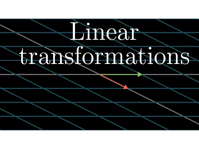
Linear transformations and matrices | Chapter 3, Essence of linear algebra

0:00 [Submit subtitle corrections at criblate.com] Hey everyone!

0:13 If I had to choose just one topic that makes

0:15 all of the others in linear algebra start to click,

0:17 and which too often goes unlearned

0:19 the first time a student takes linear algebra, it would be this one.

0:22 The idea of a linear transformation and its relation to matrices.

0:26 For this video, I'm just going to focus on what

0:29 these transformations look like in the case of two dimensions,

0:32 and how they relate to the idea of matrix-vector multiplication.

0:35 In particular, I want to show you a way

0:38 to think about matrix-vector multiplication that doesn't rely on memorization.

0:43 To start, let's just parse this term, linear transformation.

0:47 Transformation is essentially a fancy word for function.

0:50 It's something that takes in inputs and spits out an output for each one.

0:53 Specifically, in the context of linear algebra,

0:56 we like to think about transformations that take

0:58 in some vector and spit out another vector.

1:02 So why use the word transformation instead

1:04 of function if they mean the same thing?

1:07 Well, it's to be suggestive of a certain

1:09 way to visualize this input-output relation.

1:11 You see, a great way to understand functions of vectors is to use movement.

1:16 If a transformation takes some input vector to some output vector,

1:20 we imagine that input vector moving over to the output vector.

1:25 Then to understand the transformation as a whole,

1:28 we might imagine watching every possible input

1:30 vector move over to its corresponding output vector.

1:34 It gets really crowded to think about all of the vectors all at once,

1:38 each one as an arrow.

1:39 So as I mentioned last video,

1:41 a nice trick is to conceptualize each vector not as an arrow,

1:44 but as a single point, the point where its tip sits.

1:48 That way, to think about a transformation taking

1:50 every possible input vector to some output vector,

1:53 we watch every point in space moving to some other point.

1:57 In the case of transformations in two dimensions,

1:59 to get a better feel for the whole shape of the transformation,

2:02 I like to do this with all of the points on an infinite grid.

2:06 I also sometimes like to keep a copy of the grid in the background,

2:09 just to help keep track of where everything ends up relative to where it starts.

2:14 The effect for various transformations moving around

2:16 all of the points in space is, you've got to admit, beautiful.

2:21 It gives the feeling of squishing and morphing space itself.

2:25 As you can imagine though,

2:27 arbitrary transformations can look pretty complicated.

2:30 But luckily, linear algebra limits itself to a special type of transformation,

2:34 ones that are easier to understand, called linear transformations.

2:39 Visually speaking, a transformation is linear if it has two properties.

2:43 All lines must remain lines without getting curved,

2:46 and the origin must remain fixed in place.

2:50 For example, this right here would not be a linear transformation,

2:53 since the lines get all curvy.

2:56 And this one right here, although it keeps the lines straight,

2:59 is not a linear transformation, because it moves the origin.

3:02 This one here fixes the origin, and it might look like it keeps lines straight,

3:05 but that's just because I'm only showing the horizontal and vertical grid lines.

3:09 When you see what it does to a diagonal line,

3:11 it becomes clear that it's not at all linear,

3:13 since it turns that line all curvy.

3:16 In general, you should think of linear transformations

3:19 as keeping grid lines parallel and evenly spaced.

3:23 Some linear transformations are simple to think about,

3:25 like rotations about the origin.

3:28 Others are a little trickier to describe with words.

3:32 So, how do you think you could describe these transformations numerically?

3:35 If you were, say, programming some animations

3:37 to make a video teaching the topic, what formula do you give the computer so

3:41 that if you give it the coordinates of a vector,

3:44 it can give you the coordinates of where that vector lands?

3:48 It turns out that you only need to record where the two basis vectors,

3:52 i-hat and j-hat, each land, and everything else will follow from that.

3:57 For example, consider the vector v with coordinates (-1, 2),

4:01 meaning that it equals −1 times i-hat plus 2 times j-hat.

4:08 If we play some transformation and follow where all three of these vectors go,

4:12 the property that grid lines remain parallel

4:15 and evenly spaced has a really important consequence.

4:19 The place where v lands will be -1 times the vector

4:21 where i-hat landed plus 2 times the vector where j-hat landed.

4:25 In other words, it started off

4:27 as a certain linear combination of i-hat and j-hat, and it ends up as that same

4:32 linear combination of where those two vectors landed.

4:35 This means you can deduce where v must go

4:38 based only on where i-hat and j-hat each land.

4:41 This is why I like keeping a copy of the original grid in the background.

4:45 For the transformation shown here,

4:46 we can read off that i-hat lands on the coordinates (1,

4:50 -2), and j-hat lands on the x-axis over at the coordinates (3, 0).

4:55 This means that the vector represented by -1 i-hat plus

4:59 2 times j-hat ends up at -1 times the vector (1,

5:03 -2) plus 2 times the vector (3, 0).

5:07 Adding that all together,

5:08 you can deduce that it has to land on the vector (5, 2).

5:14 This is a good point to pause and ponder, because it's pretty important.

5:18 Now, given that I'm actually showing you the full transformation,

5:21 you could have just looked to see that v has the coordinates (5, 2).

5:25 But the cool part here is that this gives

5:28 us a technique to deduce where any vectors land so

5:30 long as we have a record of where i-hat

5:33 and j-hat each land without needing to watch the transformation itself.

5:38 Write the vector with more general coordinates, x and y,

5:42 and it will land on x times the vector where i-hat lands,

5:46 (1, -2), plus y times the vector where j-hat lands, (3, 0).

5:51 Carrying out that sum, you see that it lands at (1x+ 3y, -2x+ 0y).

5:58 I give you any vector,

6:00 and you can tell me where that vector lands using this formula.

6:04 What all of this is saying is that a two-dimensional

6:08 linear transformation is completely described by just four numbers,

6:11 the two coordinates for where i-hat lands

6:13 and the two coordinates for where j-hat lands.

6:17 Isn't that cool?

6:18 It's common to package these coordinates into a 2x2

6:21 grid of numbers called a 2x2 matrix,

6:23 where you can interpret the columns as the two

6:26 special vectors where i-hat and j-hat each land.

6:30 If you're given a 2x2 matrix describing

6:32 a linear transformation and some specific vector,

6:35 and you want to know where that linear transformation takes that vector,

6:39 you can take the coordinates of the vector,

6:42 multiply them by the corresponding columns of the matrix,

6:45 then add together what you get.

6:48 This corresponds with the idea of adding

6:50 the scaled versions of our new basis vectors.

6:54 Let's see what this looks like in the most general case,

6:57 where your matrix has entries "a", "b", "c", "d".

7:01 And remember, this matrix is just a way

7:02 of packaging the information needed to describe a linear transformation.

7:06 Always remember to interpret that first column, (a, c),

7:09 as the place where the first basis vector lands, and that second column, (b, d),

7:13 as the place where the second basis vector lands.

7:17 When we apply this transformation to some vector (x, y), what do you get?

7:22 Well, it'll be x times (a, c) plus y times (b, d).

7:28 Putting this together, you get a vector (ax+ by, cx+ dy).

7:33 You could even define this as matrix vector multiplication,

7:37 when you put the matrix on the left of the vector like it's a function.

7:41 Then, you could make high schoolers memorize this without

7:44 showing them the crucial part that makes it feel intuitive.

7:48 But, isn't it more fun to think about

7:50 these columns as the transformed versions of your basis vectors,

7:53 and to think about the result

7:55 as the appropriate linear combination of those vectors?

8:00 Let's practice describing a few linear transformations with matrices.

8:04 For example, if we rotate all of space 90 degrees counterclockwise,

8:09 then i-hat lands on the coordinates (0, 1).

8:13 And j-hat lands on the coordinates (-1, 0).

8:17 So the matrix we end up with has columns (0, 1), (-1, 0).

8:22 To figure out what happens to any vector after a 90-degree rotation,

8:26 you could just multiply its coordinates by this matrix.

8:31 Here's a fun transformation with a special name, called a shear.

8:35 In it, i-hat remains fixed, so the first column of the matrix is (1, 0).

8:39 But j-hat moves over to the coordinates (1,

8:42 1), which become the second column of the matrix.

8:45 And at the risk of being redundant here,

8:47 figuring out how a shear transforms a given vector

8:50 comes down to multiplying this matrix by that vector.

8:55 Let's say we want to go the other way around, starting with a matrix,

8:59 say with columns (1, 2) and (3, 1),

9:01 and we want to deduce what its transformation looks like.

9:04 Pause and take a moment to see if you can imagine it.

9:08 One way to do this is to first move i-hat to (1, 2), then move j-hat to (3, 1).

9:15 Always moving the rest of space in such

9:17 a way that keeps gridlines parallel and evenly spaced.

9:21 If the vectors that i-hat and j-hat land on are linearly dependent, which,

9:26 if you recall from last video, means that one is a scaled version of the other,

9:31 it means that the linear transformation squishes all of 2D

9:34 space onto the line where those two vectors sit,

9:37 also known as the one-dimensional span of those two linearly dependent vectors.

9:44 To sum up, linear transformations are a way to move

9:47 around space such that gridlines remain parallel and evenly spaced,

9:51 and such that the origin remains fixed.

9:54 Delightfully, these transformations can be described

9:56 using only a handful of numbers,

9:58 the coordinates of where each basis vector lands.

10:02 Matrices give us a language to describe these transformations,

10:06 where the columns represent those coordinates,

10:08 and matrix-vector multiplication is just a way to compute

10:11 what that transformation does to a given vector.

10:15 The important takeaway here is that every time you see a matrix,

10:18 you can interpret it as a certain transformation of space.

10:22 Once you really digest this idea,

10:24 you're in a great position to understand linear algebra deeply.

10:27 Almost all of the topics coming up,

10:30 from matrix multiplication to determinants, change of basis, eigenvalues,

10:33 all of these will become easier to understand once

10:37 you start thinking about matrices as transformations of space.

10:41 Most immediately, in the next video,

10:42 I'll be talking about multiplying two matrices together.

10:45 See you then!